Outline
Data
First, let’s import the necessary packages
import os
os.environ['TF_CPP_MIN_LOG_LEVEL'] = '2'
# 0 = all messages are logged (default behavior)
# 1 = INFO messages are not printed
# 2 = INFO and WARNING messages are not printed
# 3 = INFO, WARNING, and ERROR messages are not printed

import tensorflow as tf
import pandas as pd
import numpy as np
import matplotlib.pyplot as plt

from tensorflow.keras.utils import to_categorical, plot_model
from scipy.ndimage import convolve
from keras.models import Model
from keras.layers import Input, Dense, Layer, Conv2D, MaxPool2D, Flatten
from keras.losses import Loss
Next, download the MNIST Dataset.
The MNIST dataset comprises images of handwritten digits from 0 to 9. In the dataset, the first column contains the label of the image (i.e., the digit it represents), while the remaining 784 columns (corresponding to 28 x 28 pixels) hold the pixel values of the image.
To visualize the images, we need to reshape the 784 columns back into a 28 x 28 pixel matrix and then plot them:
def show_img(data):
    # show figures in the dataset
    fig = plt.figure(figsize = (24,3))
    plt.imshow(data.reshape(28,28) , cmap = plt.get_cmap('gray'))
    plt.show()
train = pd.read_csv('data/mnist_train_small.csv')
train.head(3)
| label | 1x1 | 1x2 | 1x3 | 1x4 | 1x5 | 1x6 | ... | 28x24 | 28x25 | 28x26 | 28x27 | 28x28 | |
|---|---|---|---|---|---|---|---|---|---|---|---|---|---|
| 0 | 6 | 0 | 0 | 0 | 0 | 0 | 0 | ... | 0 | 0 | 0 | 0 | 0 |
| 1 | 5 | 0 | 0 | 0 | 0 | 0 | 0 | ... | 0 | 0 | 0 | 0 | 0 |
| 2 | 7 | 0 | 0 | 0 | 0 | 0 | 0 | ... | 0 | 0 | 0 | 0 | 0 |
3 rows × 785 columns
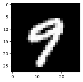
# drop label column and select a row
img = train.drop('label', axis = 1).iloc[80]
img = np.array(img)

show_img(img)
Convolutions
First, let’s understand what is Convolutions. Convolution is a mathematical operation that involves sliding a small matrix, known as a kernel or filter, across a larger matrix representing the input data, such as an image. During this process, the element-wise product $\odot$ is computed between the kernel and each local region (sub-matrix) it covers on the input data matrix. The result of this operation is a new matrix, called a feature map, which encodes information about the presence, absence, or strength of specific features in the input data.
Let’s examine the following convolutional operations to illustrate this concept.
One Dimensional Convolutions
Let’s consider $\mathbf{x}$ as an input vector with $n$ elements and $\mathbf{w}$ as a weight vector, also known as a filter, with $k \leq n$.
\[\mathbf{x} = \left( \begin{array}{c} x_{1}\\ x_{2}\\ \vdots\\ x_{n} \end{array} \right), ~~~~ \mathbf{w} = \left( \begin{array}{c} w_{1}\\ w_{2}\\ \vdots\\ w_{k} \end{array} \right)\]Here $k$ is known as the window size and indicates the size of the filter applied to the input vector $\mathbf{x}$. It defines the region of the local neighborhood within the input vector $\mathbf{x}$ used for computing output values. To proceed, we define a subvector of $\mathbf{x}$ with the same size as the filter vector. Let $\mathbf{x}_k(i)$ denote the window of $\mathbf{x}$ of size $k$ starting at position $i$:
\[\mathbf{x}_k(i) = \left( \begin{array}{c} x_i \\ x_{i+1} \\ \vdots\\ x_{i+k-1} \end{array} \right).\]For $k \leq n$, it must be that $i+k-1 \leq n$, implying $1 \leq i \leq n-k+1$. As a validity test, if we start at $i = n-k+1$, then the end position is $i+k-1 = n$. If we calculate the total number of elements by the difference in position provides the window size $k$, confirmed by $n - i = n - (n-k+1) = k$. For example, with $n = 5$ and $k = 3$:
\[\mathbf{x} = \left( \begin{array}{c} x_{1}\\ x_{2}\\ x_{3}\\ x_{4}\\ x_{5} \end{array} \right), ~~~~ \mathbf{w} = \left( \begin{array}{c} w_{1}\\ w_{2}\\ w_{3} \end{array} \right)\]the window of $\mathbf{x}$ from $i = 2$ to $i+k-1 = 4$ is:
\[\mathbf{x}_3(2) = \left( \begin{array}{c} x_2 \\ x_{3}\\ x_{4} \end{array} \right)\]Example
Let’s first consider a particular example with input vector $\mathbf{x}$ of size $n = 5$ and a weight vector with window size $k = 3$. The vectors are illustrated in the following figure:
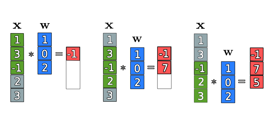
The convolution steps for the sliding windows of $\mathbf{x}$ with the filter $\mathbf{w}$ are:
\[\sum \mathbf{x}_3(1) \odot \mathbf{w} = \sum (1, 3, -1)^T \odot (1, 0, 2)^T = \sum (1 \cdot 1, 3 \cdot 0, -1 \cdot 2) = 1 + 0 - 2 = -1,\] \[\sum \mathbf{x}_3(2) \odot \mathbf{w} = \sum (3, -1, 2)^T \odot (1, 0, 2)^T = \sum (3 \cdot 1, -1 \cdot 0, 2 \cdot 2) = 3 + 0 + 4 = 7,\] \[\sum \mathbf{x}_3(3) \odot \mathbf{w} = \sum (-1, 2, 3)^T \odot (1, 0, 2)^T = \sum (-1 \cdot 1, 2 \cdot 0, 3 \cdot 2) = -1 + 0 + 6 = 5.\]The element-wise product $\odot$ , also known as the Hadamard product, multiplies corresponding elements in two vectors. Unlike the typical inner product, which multiplies an element by a column, this operation multiplies an element by its corresponding element in another vector. This steps provide the convolution between the two vectors resulting in a vector of size n-k+1 = 3. Thus, the convolution $\mathbf{x} * \mathbf{w}$ is:
\[\mathbf{x} * \mathbf{w} = \left( \begin{array}{c} -1\\ 7\\ 5 \end{array} \right)\]# Code for the example
X = np.array([1, 3, -1, 2, 3])
# flip the filter W to use the convolve function
# as expected in machine learning and deep learning context
W = np.flip(np.array([1, 0, 2]))
# perform 1D convolution
output = np.convolve(X, W, mode='valid')
print("Input vector X:", X.shape)
print("filter W:", W.shape)
print("output X*W:", output)
Input vector X: (5,)
filter W: (3,)
output X*W: [-1  7  5]
This demonstrates that convolution is an element-wise product between a subvector and a weight vector of the same size, providing a scalar value when summed, which forms the result of the convolution operation.
To simplify the notation, let’s adopt the convention that for a vector $\mathbf{a} \in \mathbb{R}^k$, define the summation operator as one that adds all elements of the vector. That is,
\[\text{Sum}(\mathbf{a}) = \sum_{i=1}^{k} a_{i}.\]From the example, we would have
\[\sum \mathbf{x}_3(1) \odot \mathbf{w} = \text{Sum}\bigg( \mathbf{x}_3(1) \odot \mathbf{w} \bigg)= 1 + 0 - 2 = -1.\]Then, we can define a general one dimensional convolution operation between $\mathbf{x}$ and $\mathbf{w}$, denoted by the asterisk symbol $\ast$, as
\[{\small \mathbf{x} \ast \mathbf{w} = \left( \begin{array}{c} \text{Sum}(\mathbf{x}_k(1) \odot \mathbf{w})\\ \vdots\\ \text{Sum}(\mathbf{x}_k(i) \odot \mathbf{w})\\ \vdots\\ \text{Sum}(\mathbf{x}_k(n-k+1) \odot \mathbf{w}) \end{array} \right). }\]The convolution of $\mathbf{x} \in \mathbf{R}^{n}$ and $\mathbf{W} \in \mathbf{R}^{k}$ results in a vector of size $n-k+1$. The i-th element from this output vector can be decomposed as
\[\text{Sum}(\mathbf{x_k}(i) \odot \mathbf{w}) = x_{i}w_1 + x_{i+1}w_2 + \cdots + x_{(i+k-1)}w_k = \sum_{j=1}^{k} x_{(i+j-1)}w_j.\]This shows that the sum is over all elements of the subvector $\mathbf{x}_k(i)$, so the last element of this sum must coincide with the last elements of $\mathbf{x}_k(i)$ and $\mathbf{w}$. This results in the convolution of $\mathbf{x}$ with $\mathbf{w}$ over the window defined by $k$.
Two Dimensional Convolutions
We can extend the convolution operation to an matrix input instead of a vector. Let $\mathbf{X}$ be an input matrix with $n \times n$ elements and $\mathbf{W}$ be the weight matrix, also known as a filter, with $k \leq n$.
\[\mathbf{X} = \begin{bmatrix} x_{1,1} & x_{1,2} & \cdots & x_{1,n} \\ x_{2,1} & x_{2,2} & \cdots & x_{2,n} \\ \vdots & \vdots & \ddots & \vdots \\ x_{n,1} & x_{n,2} & \cdots & x_{n,n} \end{bmatrix},~~ \mathbf{W}=\begin{bmatrix} w_{1,1} & w_{1,2} & \cdots & w_{1,k} \\ w_{2,1} & w_{2,2} & \cdots & w_{2,k} \\ \vdots & \vdots & \ddots & \vdots \\ w_{k,1} & w_{k,2} & \cdots & w_{k,k} \end{bmatrix}\]Here, similar to the one dimensional case, $k$ is the window size and indicates the size of the filter applied to the input matrix $\mathbf{X}$. From the one dimensional case we can extend the notion of a sub vector to a sub matrix. Let $\mathbf{X}_k(i,j)$ denote the $k \times k$ submatrix of $\mathbf{X}$ starting at row $i$ and column $j$ as
\[\mathbf{X}_k(i,j) = \begin{bmatrix} x_{i,j} & x_{i,~(j+1)} & \cdots & x_{i,~(j+k-1)} \\ x_{(i+1),~j} & x_{(i+2),~j} & \cdots & x_{(i+1), (j+k-1)} \\ \vdots & \vdots & \ddots & \vdots \\ x_{(i+k-1), ~j} & x_{(i+1),(j+1)} & \cdots & x_{(i+k-1),(j+k-1)} \end{bmatrix}\]where for two indices, give that this is a square matrix, the range is simple $1 \leq (i,j) \leq n-k+1$.
As for the one dimensional case, to simplify the notation, we adopt the convention that for a matrix $\mathbf{A} \in \mathbb{R}^{k \times k}$ define the summation operator as one that adds all elements of the matrix.
\[\text{Sum}(\mathbf{A}) = \sum_{i=1}^{k}\sum_{j=1}^{k} a_{i,j}\]Then, we can define a general two dimensional convolution operation between matrices $\mathbf{X}$ and $\mathbf{W}$, as
\[{\small \mathbf{X} \ast \mathbf{W} = \begin{bmatrix} \text{Sum}(x_k(1,1) \odot \mathbf{W}) & \cdots & \text{Sum}(x_k(1,n-k+1) \odot \mathbf{W}) \\ \text{Sum}(x_k(2,1) \odot \mathbf{W}) & \cdots &\text{Sum}(x_k(2,n-k+1) \odot \mathbf{W})\\ \vdots & \ddots & \vdots \\ \text{Sum}(x_k(n-k+1,1) \odot \mathbf{W}) & \cdots & \text{Sum}(x_k(n-k+1,n-k+1) \odot \mathbf{W}) \end{bmatrix} }\]where
\[\text{Sum}(\mathbf{X}_k(i,j) \odot \mathbf{W})=\sum_{a=1}^{k}\sum_{b=1}^{k} x_{(i+a-1),(j+b-1)} w_{a,b}\]The convolution of $\mathbf{X} \in \mathbf{R}^{n \times n}$ and $\mathbf{W} \in \mathbf{R}^{k \times k}$ results in a $(n-k+1) \times (n-k+1)$ matrix.
Example
Let’s consider a particular example with input matrix $\mathbf{X}$ with dimension $3 \times 3$ (n = 3) and a weight matrix with dimension $2 \times 2$ (k = 2). The matrices are illustrated in the following figure:
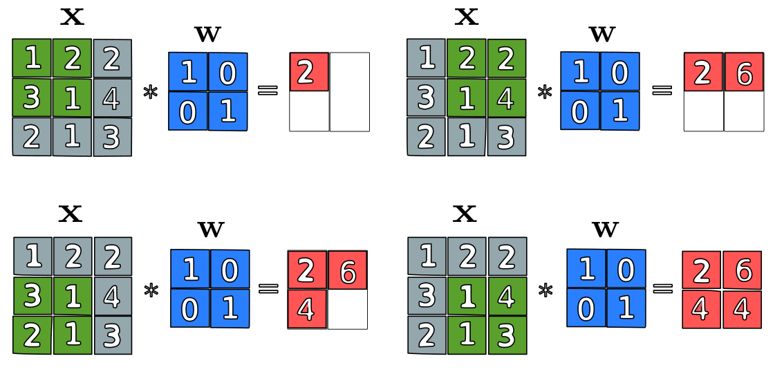
The convolution steps for the sliding windows of $\mathbf{X}$ with the filter $\mathbf{W}$ illustrated in the figure are mathematically translated to:
\[\text{Sum}(\mathbf{X}_k(1,1) \odot \mathbf{W})=\text{Sum}\bigg( \begin{bmatrix} 1 & 2 \\ 3 & 1 \end{bmatrix} \odot \begin{bmatrix} 1 & 0 \\ 0 & 1 \end{bmatrix} \bigg) = 2\] \[\text{Sum}(\mathbf{X}_2(1,2) \odot \mathbf{W}) = \text{Sum}\bigg( \begin{bmatrix} 2 & 2 \\ 1 & 4 \end{bmatrix} \odot \begin{bmatrix} 1 & 0 \\ 0 & 1 \end{bmatrix} \bigg)= 6\] \[\text{Sum}(\mathbf{X}_2(2,1) \odot \mathbf{W}) = \text{Sum}\bigg( \begin{bmatrix} 3 & 1 \\ 2 & 1 \end{bmatrix} \odot \begin{bmatrix} 1 & 0 \\ 0 & 1 \end{bmatrix} \bigg)= 4\] \[\text{Sum}(\mathbf{X}_2(2,2) \odot \mathbf{W}) = \text{Sum}\bigg( \begin{bmatrix} 1 & 4 \\ 3 & 3 \end{bmatrix} \odot \begin{bmatrix} 1 & 0 \\ 0 & 1 \end{bmatrix} \bigg) = 4\]The convolution $\mathbf{X}*\mathbf{W}$ has size $2 \times 2$, since $n - k + 1 = 3 - 2 + 1 = 2$, and is given by
\[\mathbf{X}*\mathbf{W} = \begin{bmatrix} \text{Sum}(\mathbf{X}_2(1,1) \odot \mathbf{W}) & \text{Sum}(\mathbf{X}_2(1,2) \odot \mathbf{W}) \\ \\ \text{Sum}(\mathbf{X}_2(2,1) \odot \mathbf{W}) & \text{Sum}(\mathbf{X}_2(2,2) \odot \mathbf{W}) \end{bmatrix} = \begin{bmatrix} 2 & 6 \\ 4 & 4 \end{bmatrix}\]Three dimensional Convolution on CNNs
We now extend the convolution operation to a three-dimensional matrix, also called a rank-3 tensor. The first dimension comprises the rows (height), second dimension the columns (width) and the third dimension the channels (number of 2D slices stacked along the depth axis). Typically in CNNs, we use a 3D filter $\mathbf{W} \in \mathbb{R}^{k \times k \times m}$, with the number of channels equal to the number of channels of the input tensor $\mathbf{X} \in \mathbb{R}^{n \times n \times m}$, in this case with $m$ channels each. Mathematically we represent as:
\[\mathbf{X}= \begin{bmatrix} \begin{bmatrix} x_{1,1,1} & x_{1,2,1} & \cdots & x_{1,n,1} \\ x_{2,1,1} & x_{2,2,1} & \cdots & x_{2,n,1} \\ \vdots & \vdots & \ddots & \vdots \\ x_{n,1,1} & x_{n,2,1} & \cdots & x_{n,n,1} \end{bmatrix}\\ \\ \begin{bmatrix} x_{1,1,2} & x_{1,2,2} & \cdots & x_{1,n,2} \\ x_{2,1,2} & x_{2,2,2} & \cdots & x_{2,n,2} \\ \vdots & \vdots & \ddots & \vdots \\ x_{n,1,2} & x_{n,2,2} & \cdots & x_{n,n,2} \end{bmatrix}\\ \\ \vdots\\ \\ \begin{bmatrix} x_{1,1,m} & x_{1,2,m} & \cdots & x_{1,n,m} \\ x_{2,1,m} & x_{2,2,m} & \cdots & x_{2,n,m} \\ \vdots & \vdots & \ddots & \vdots \\ x_{n,1,m} & x_{n,2,m} & \cdots & x_{n,n,m} \end{bmatrix} \end{bmatrix},~~ \mathbf{W}= \begin{bmatrix} \begin{bmatrix} w_{1,1,1} & w_{1,2,1} & \cdots & w_{1,k,1} \\ w_{2,1,1} & w_{2,2,1} & \cdots & w_{2,k,1} \\ \vdots & \vdots & \ddots & \vdots \\ w_{k,1,1} & w_{k,2,1} & \cdots & w_{k,k,1} \end{bmatrix}\\ \\ \begin{bmatrix} w_{1,1,2} & w_{1,2,2} & \cdots & w_{1,k,2} \\ w_{2,1,2} & w_{2,2,2} & \cdots & w_{2,k,2} \\ \vdots & \vdots & \ddots & \vdots \\ w_{k,1,2} & w_{k,2,2} & \cdots & w_{k,k,2} \end{bmatrix} \\ \vdots\\ \\ \begin{bmatrix} w_{1,1,r} & w_{1,2,r} & \cdots & w_{1,k,m} \\ w_{2,1,r} & w_{2,2,r} & \cdots & w_{2,k,m} \\ \vdots & \vdots & \ddots & \vdots \\ w_{k,1,r} & w_{k,2,r} & \cdots & w_{k,k,m} \end{bmatrix} \end{bmatrix}\]Similar to convolutions in other dimensions, the window size must satisfy $k \leq n$, and the total number of slice matrices along the depth of the filter and input tensor are fixed as $m$. This mathematical representation of a tensor may seem complex at first, but it closely resembles how Python libraries like NumPy represent a tensor, with exception of the order of rows, columns and depth.
When defining a sub-tensor from the input tensor $\mathbf{X}$, let $\mathbf{X}_k(i,j)$ denote a $k \times k \times m$ sub-tensor of $\mathbf{X}$ that starts at row $i$, column $j$, and encompasses the full depth $m$ of the input. In the context where the filter spans the entire depth of the input (i.e., the number of channels $r$ in the filter is equal to the depth $m$ of the input), the depth index $q$ is not needed because the filter processes all depth layers simultaneously. Therefore, the sub-tensor $\mathbf{X}_k(i,j)$ is defined as follows:
\[{\small \mathbf{X}_k(i,j,q = m)= \mathbf{X}_k(i,j) = \begin{bmatrix} \begin{bmatrix} x_{i,j,1} & x_{i,(j+1),1} & \cdots & x_{i,(j+k-1),1} \\ x_{(i+1),j,1} & x_{(i+1),(j+1),1} & \cdots & x_{(i+1),(j+k-1),1} \\ \vdots & \vdots & \ddots & \vdots \\ x_{(i+k-1),j,1} & x_{(i+k-1),(j+1),1} & \cdots & x_{(i+k-1),(j+k-1),1} \end{bmatrix}\\ \\ \\ \begin{bmatrix} x_{i,j,2} & x_{i,(j+1),2} & \cdots & x_{i,(j+k-1),2} \\ x_{(i+1),j,2} & x_{(i+1),(j+1),2} & \cdots & x_{(i+1),(j+k-1),2} \\ \vdots & \vdots & \ddots & \vdots \\ x_{(i+k-1),j,2} & x_{(i+k-1),(j+1),2} & \cdots & x_{(i+k-1),(j+k-1),2} \end{bmatrix}\\ \\ \vdots\\ \\ \begin{bmatrix} x_{i,j,m} & x_{i,(j+1),m} & \cdots & x_{i,(j+k-1),m} \\ x_{(i+1),j,m} & x_{(i+1),(j+1),m} & \cdots & x_{2,n,m} \\ \vdots & \vdots & \ddots & \vdots \\ x_{(i+k-1),j,m} & x_{(i+k-1),(j+1),m} & \cdots & x_{(i+k-1),(j+k-1),m} \end{bmatrix} \end{bmatrix} }\]The indices from the subtensor for rows and columns range from $1 \leq (i,j) \leq n-k+1$, where $n$ is the dimension of the input $\mathbf{X}$ and $k$ is the window size of the filter $\mathbf{W}$, consistent with two-dimensional convolutions. The depth dimension is fixed at $m$, so it’s redundant carrying $q = m$ in our notation.
As in the case of convolution in lower dimensions, we define the summation operator as one that adds all elements within the tensor. Therefore, given a tensor $\mathbf{A} \in \mathbb{R}^{k \times k \times m}$, the summation operation is defined as:
\[\text{Sum}(\mathbf{A}) = \sum_{a=1}^{k}\sum_{b=1}^{k}\sum_{q=1}^{m}a_{ijq}\]This summation adds up all the elements in the tensor $\mathbf{A}$, where $a_{ijq}$ denotes the element located at the $i$-th row, $j$-th column, and $q$-th depth layer.
Before we generalize the convolution operation to three dimensions, let’s consider an example to illustrate the logic behind this mathematical notation and how it translates to the operations performed in a CNN.
Example
Consider a input tensor $\mathbf{X}$ with dimension $3 \times 3 \times 3$ (n = 3 and m = 3 channels) and a filter with dimension $2 \times 2 \times 3$ ( windows size with k = 2 and m = 3 channels). The tensors are illustrated in the following figure:
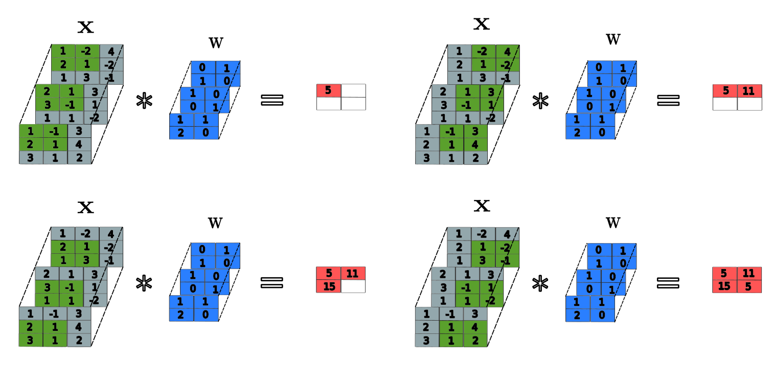
The convolution steps for the sliding windows of $\mathbf{X}$ with the filter $\mathbf{W}$ illustrated in the figure are:
\[{\small \text{Sum}(\mathbf{X}_2(1,1) \odot \mathbf{W}) = \text{Sum}\bigg( \begin{bmatrix} \begin{bmatrix} 1 & -1 \\ 2 & 1 \end{bmatrix} \\ \\ \begin{bmatrix} 2 & 1 \\ 3 & -1 \end{bmatrix} \\ \\ \begin{bmatrix} 1 & -2 \\ 2 & 1 \end{bmatrix} \end{bmatrix} \odot \begin{bmatrix} \begin{bmatrix} 1 & 1 \\ 2 & 0 \end{bmatrix} \\ \\ \begin{bmatrix} 1 & 0 \\ 0 & 1 \end{bmatrix} \\ \\ \begin{bmatrix} 0 & 1 \\ 1 & 0 \end{bmatrix} \end{bmatrix} \bigg) = \text{Sum}\bigg( \begin{bmatrix} \begin{bmatrix} 1 & -1 \\ 4 & 0 \end{bmatrix} \\ \\ \begin{bmatrix} 2 & 0 \\ 0 & -1 \end{bmatrix} \\ \\ \begin{bmatrix} 0 & -2 \\ 2 & 0 \end{bmatrix} \end{bmatrix} \bigg) = 5 }\] \[{\small \text{Sum}(\mathbf{X}_2(1,2) \odot \mathbf{W}) = \text{Sum}\bigg( \begin{bmatrix} \begin{bmatrix} -1 & 3 \\ 1 & -4 \end{bmatrix} \\ \\ \begin{bmatrix} 1 & 3 \\ -1 & 1 \end{bmatrix} \\ \\ \begin{bmatrix} -2 & 4 \\ 1 & -2 \end{bmatrix} \end{bmatrix} \odot \begin{bmatrix} \begin{bmatrix} 1 & 1 \\ 2 & 0 \end{bmatrix} \\ \\ \begin{bmatrix} 1 & 0 \\ 0 & 1 \end{bmatrix} \\ \\ \begin{bmatrix} 0 & 1 \\ 1 & 0 \end{bmatrix} \end{bmatrix} \bigg) = \text{Sum}\bigg( \begin{bmatrix} \begin{bmatrix} -1 & 3 \\ 2 & 0 \end{bmatrix} \\ \\ \begin{bmatrix} 1 & 0 \\ 0 & 1 \end{bmatrix} \\ \\ \begin{bmatrix} 0 & 4 \\ 1 & 0 \end{bmatrix} \end{bmatrix} \bigg) = 11 }\] \[{\small \text{Sum}(\mathbf{X}_2(2,1) \odot \mathbf{W}) = \text{Sum}\bigg( \begin{bmatrix} \begin{bmatrix} 2 & 1 \\ 3 & 1 \end{bmatrix} \\ \\ \begin{bmatrix} 3 & -1 \\ 1 & 1 \end{bmatrix} \\ \\ \begin{bmatrix} 2 & 1 \\ 1 & 3 \end{bmatrix} \end{bmatrix} \odot \begin{bmatrix} \begin{bmatrix} 1 & 1 \\ 2 & 0 \end{bmatrix} \\ \\ \begin{bmatrix} 1 & 0 \\ 0 & 1 \end{bmatrix} \\ \\ \begin{bmatrix} 0 & 1 \\ 1 & 0 \end{bmatrix} \end{bmatrix} \bigg) = \text{Sum}\bigg( \begin{bmatrix} \begin{bmatrix} 2 & 1 \\ 6 & 0 \end{bmatrix} \\ \\ \begin{bmatrix} 3 & 0 \\ 0 & 1 \end{bmatrix} \\ \\ \begin{bmatrix} 0 & 1 \\ 1 & 0 \end{bmatrix} \end{bmatrix} \bigg) = 15 }\] \[{\small \text{Sum}(\mathbf{X}_2(2,2) \odot \mathbf{W}) = \text{Sum}\bigg( \begin{bmatrix} \begin{bmatrix} 1 & 4 \\ 1 & 2 \end{bmatrix} \\ \\ \begin{bmatrix} -1 & 1 \\ 1 & -2 \end{bmatrix} \\ \\ \begin{bmatrix} 1 & -2 \\ 3 & -1 \end{bmatrix} \end{bmatrix} \odot \begin{bmatrix} \begin{bmatrix} 1 & 1 \\ 2 & 0 \end{bmatrix} \\ \\ \begin{bmatrix} 1 & 0 \\ 0 & 1 \end{bmatrix} \\ \\ \begin{bmatrix} 0 & 1 \\ 1 & 0 \end{bmatrix} \end{bmatrix} \bigg) = \text{Sum}\bigg( \begin{bmatrix} \begin{bmatrix} 1 & 4 \\ 2 & 0 \end{bmatrix} \\ \\ \begin{bmatrix} -1 & 0 \\ 0 & -2 \end{bmatrix} \\ \\ \begin{bmatrix} 0 & -2 \\ 3 & 0 \end{bmatrix} \end{bmatrix} \bigg) = 5 }\]The convolution $\mathbf{X}*\mathbf{W}$ has size $2 \times 2$, since $n - k + 1 = 3 - 2 + 1 = 2$, and $m = 3$; it is is given as
\[\mathbf{X}*\mathbf{W} = \begin{bmatrix} \text{Sum}(\mathbf{X}_2(1,1) \odot \mathbf{W}) & \text{Sum}(\mathbf{X}_2(1,2) \odot \mathbf{W}) \\ \\ \text{Sum}(\mathbf{X}_2(2,1) \odot \mathbf{W}) & \text{Sum}(\mathbf{X}_2(2,2) \odot \mathbf{W}) \end{bmatrix} = \begin{bmatrix} 5 & 11 \\ 15 & 5 \end{bmatrix}\]X = np.array([
[[1, -1, 3],
[2, 1, 4],
[3, 1, 2]],
[[2, 1, 3],
[3, -1, 1],
[1, 1, -2]],
[[1, -2, 4],
[2, 1, -2],
[1, 3, -1]]
], dtype=np.float32)
# TensorFlow expects the input to have a shape of [batch, (depth, height, width), channels]
# Add a batch dimension and a channel dimension to X
X = X.reshape(1, *X.shape, 1)
# create a simple 3D kernel
W = np.array([
[[1, 1],
[2, 0]],
[[1, 0],
[0, 1]],
[[0, 1],
[1, 0]]
], dtype=np.float32)
# TensorFlow expects the filter to have a shape of
# [(depth, height, width), in_channels = 1, out_channels = 1]
# Since our input has a single channel (in_channels = 1) and
# we want a single output channel ( out_channels = 1),
# Add those dimensions to W
W = W.reshape(*W.shape, 1, 1)
# 3D convolution
output = tf.nn.conv3d(input=X, filters=W, strides=[1, 1, 1, 1, 1], padding="VALID")
# squeeze to remove the redundant dimensions of batch and channel
output_2d = output.numpy().squeeze()
print("Shape of input tensor X:\n", X.shape)
print("Shape of filter tensor W:\n", W.shape)
print("Convolved output shape with channel and batch dimension:\n", output.shape)
print("Convolved output:\n", output_2d)
Shape of input tensor X:
 (1, 3, 3, 3, 1)
Shape of filter tensor W:
 (3, 2, 2, 1, 1)
Convolved output shape with channel and batch dimension:
 (1, 1, 2, 2, 1)
Convolved output:
 [[ 5. 11.]
 [15.  5.]]
When the number of channels is fixed for both tensors the result of the convolution is a matrix of two dimension, and not a tensor. The matrix from the convolution has dimension $(n-k+1) \times (n-k+1)$ and can be represented as:
\[\mathbf{X} \ast \mathbf{W} = \begin{bmatrix} \text{Sum}(X_k(1,1) \odot \mathbf{W}) & \cdots & \text{Sum}(X_k(1,n-k+1) \odot \mathbf{W}) \\ \vdots & \ddots & \vdots \\ \text{Sum}(X_k(n-k+1,1) \odot \mathbf{W}) & \cdots & \text{Sum}(X_k(n-k+1,n-k+1) \odot \mathbf{W}) \end{bmatrix}\]where
\[\begin{align*} \text{Sum}(\mathbf{X}_k(i,j) \odot \mathbf{W}) = \sum_{a=1}^{k}\sum_{b=1}^{k}\sum_{c=1}^{m}x_{(i+a-1),(j+b-1),~c}~w_{a,b,c} \end{align*}\]for $(i,j) = 1,2, \cdots, n-k+1$.
This process can be visualized as each slice of the filter $\mathbf{W}$ matching with a corresponding slice in $\mathbf{X}$, aggregating information across all channels to form a 2D matrix that represents the features extracted from the input tensor $\mathbf{X}$.
In conclusion, the channels of the input tensor $\mathbf{X}$ represent various features of the input data, and the filter $\mathbf{W}$ is used to extract these features by convolving it with $\mathbf{X}$. By using a filter with the same number of channels as the input, each channel’s features are processed, allowing the network to learn from each aspect of the input data separately.
Convolutional Layer
In a CNN, the input tensor is generally denoted as $\mathbf{X} \in \mathbb{R}^{n_0 \times n_0 \times m_0}$, where $n_0 \times n_0$ represents the spatial dimensions of a 2D input image (e.g., pixels), and $ m_0$ represents the depth, such as 1 for grayscale images or 3 for RGB color images. This input tensor is convolved with multiple filters designed to extract relevant information or features. After convolution, these feature are passed through activation functions within the convolutional layer $\mathbf{Z}^1$, which introduce non-linear properties to the model. The process then repeat itself for the subsequent convolutional layers.
To exemplify this process, consider two filters $\mathbf{W}_1$ and $\mathbf{W}_2$, which convolve with the input tensor $\mathbf{X}$ to pass the extracted features to the the convolutional layer $\mathbf{Z}^1 \in \mathbb{R}^{n_1 \times n_1 \times m_1}$:
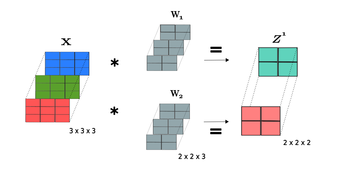
Considering a input tensor $\mathbf{X}$ with spatial dimension $n_0 = 3$ and $m_0 = 3$ channels convolved with two filters $\mathbf{W}_1$ and $\mathbf{W}_2$ with window size $k = 2$, we obtain the output tensor at layer $\mathbf{Z}^1$. the dimension of $\mathbf{Z}^1$ is $(n_0 - k + 1) \times (n_0 - k + 1) \times m_1$, resulting in a $2 \times 2 \times 2$ tensor, where $m_1 = 2$ corresponding to the number of filters applied.
Let’s incorporate the bias terms $b_1, b_2 \in \mathbb{R}$ corresponding to each filter $\mathbf{W}_1$ and $\mathbf{W}_2$, and a activation function $f(~ . ~)$. We represent a single forward step in our simplified visualization of a CNN, going from input to the subsequent layer as:
\[{\small {\mathbf{net}^1} = \begin{bmatrix} \begin{bmatrix} \text{Sum}(X_2(1,1) \odot \mathbf{W}_1)+b_1& \text{Sum}(X_2(1,2) \odot \mathbf{W}_1) +b_1 \\ \\ \text{Sum}(X_2(2,1) \odot \mathbf{W}_1)+b_1& \text{Sum}(X_2(2,2) \odot \mathbf{W}_1)+b_1 \end{bmatrix}\\ \\ \\ \begin{bmatrix} \text{Sum}(X_2(1,1) \odot \mathbf{W}_2)+b_2& \text{Sum}(X_2(1,2) \odot \mathbf{W}_2) +b_2 \\ \\ \text{Sum}(X_2(2,1) \odot \mathbf{W}_2)+b_2& \text{Sum}(X_2(2,2) \odot \mathbf{W}_2)+b_2 \end{bmatrix} \end{bmatrix} }\]The net signal after convolution is followed by the activation function to introduce non-linearity:
\[{\small {\mathbf{Z}^1} = f(\mathbf{net}^1) = \begin{bmatrix} \\ \begin{bmatrix} f(\text{Sum}(X_2(1,1) \odot \mathbf{W}_1) +b_1)& f(\text{Sum}(X_2(1,2) \odot \mathbf{W}_1)+b_1) \\ \\ f(\text{Sum}(X_2(2,1) \odot \mathbf{W}_1)+b_1)& f(\text{Sum}(X_2(2,2) \odot \mathbf{W}_1)+b_1) \end{bmatrix}\\ \\ \\ \begin{bmatrix} f(\text{Sum}(X_2(1,1) \odot \mathbf{W}_2) + b_2)& f(\text{Sum}(X_2(1,2) \odot \mathbf{W}_2) + b_2) \\ \\ f(\text{Sum}(X_2(2,1) \odot \mathbf{W}_2)+ b_2)& f(\text{Sum}(X_2(2,2) \odot \mathbf{W}_2)+ b_2) \end{bmatrix} \end{bmatrix}. }\]Resulting in the feature map, which represents the actual output of the layer after applying the activation function to the net signal. The activation function can be one commonly used in neural networks, such as identity, sigmoid, tanh, or ReLU. In the language of convolutions, this is simplified as:
\[{ \mathbf{Z}^1 } = \begin{bmatrix} f(\mathbf{X} * \mathbf{W}_1 \oplus b_1)\\ \\ f(\mathbf{X} * \mathbf{W}_2 \oplus b_2) \end{bmatrix},\]where $\oplus$ denotes the addition of the bias term to each element of the feature maps produced by $\mathbf{X} * \mathbf{W}_1$ and $\mathbf{X} * \mathbf{W}_2$. For a compact representation:
\[\large\boxed{ {\mathbf{Z}^1} = f(\mathbf{X} * \mathbf{W}_1 \oplus b_1, \mathbf{X} * \mathbf{W}_2 \oplus b_2)}\]More general case
Extending this concept to a more general and formal case, from the $l$-th layer to the $l+1$-th layer with multiple filters, we denote the tensor at layer $l$ as $\mathbf{Z}^l \in \mathbb{R}^{n_l \times n_l \times m_l} $. Each element $Z_{i,j,q}^l$ of the tensor represents the output value of a neuron located at row $i$, column $j$, and channel $q$ for layer $l$, where $1 \leq (i,j) \leq n_l$ and $1 \leq q \leq m_l = 3$. Assuming we have $m_{l+1}$ filters $ \{ \mathbf{W_1}, \cdots, \mathbf{W_{m_{l+1}}} \} $, the output feature map passed through the next layer will have $m_{l+1}$ channels. Consider the following figure:
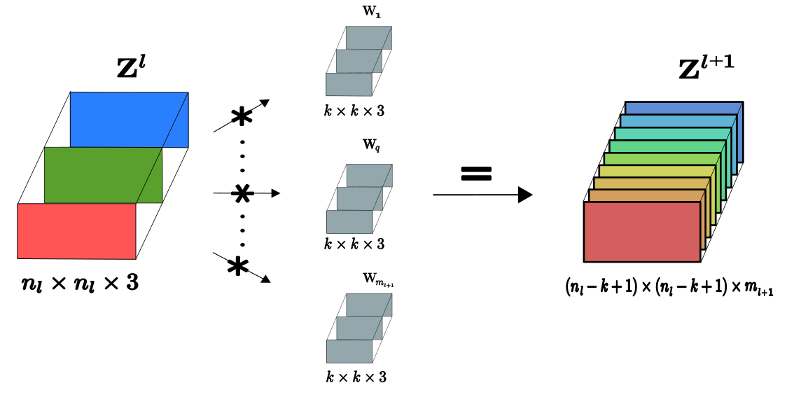
The convolution $f(\mathbf{Z}^l * \mathbf{W_q} \oplus b_q)$ for a given filter $q$ produces a feature map matrix of dimension $(n_l-k+1) \times (n_l-k+1)$, where each element of this feature map corresponds to a neuron’s output at layer $l+1$. Convolving $\mathbf{Z}^l$ with all $m_{l+1}$ filters, we form the tensor $\mathbf{Z}^{l+1}$ for layer $l+1$ with dimensions $(n_l-k+1) \times (n_l-k+1) \times m_{l+1}$. The result for this tensor at layer $l+1$ is:
\[\large\boxed{ {\mathbf{Z}^{l+1}} = f\bigg(\big(\mathbf{Z}^l * \mathbf{W}_1 \oplus b_1\big), \cdots,\big(\mathbf{Z}^l * \mathbf{W}_q \oplus b_q\big), \cdots, \big( \mathbf{Z}^l * \mathbf{W}_{m_{l+1}} \oplus b_{m_{l+1}}\big)\bigg)}\]In summary, a Convolutional Layer accepts an $n_l \times n_l \times 3$ tensor, denoted as $\mathbf{Z}^l$, from layer $l$. It proceeds to compute the tensor $\mathbf{Z}^{l+1}$, which has dimensions $n_{l+1} \times n_{l+1} \times m_{l+1}$, where $n_{l+1} = n_l - k + 1$. This computation for the subsequent layer $l+1$ involves convolving $\mathbf{Z}^l$ with $m_{l+1}$ distinct filters, each of dimension $k \times k \times 3$. Following the convolution, a bias term is added, and a nonlinear activation function $f(~.~)$ is applied to introduce nonlinearity into the model.
Padding and Striding
One of the problem with the convolution operation is that the size of the tensor will decrease in each successive layer. If a tensor $\mathbf{Z}^l$ at layer $l$ has size $n_l \times n_l \times m_l$, and we use filters of size $k \times k \times m_l$, then each channel in a layer $l+1$ will have size $(n_l - (k - 1)) \times (n_l-(k -1))$. That is, the number of rows and columns for each successive tensor will shrink by $k-1$.
Padding
Padding involves adding zeros or other values around the edges of the input data before applying a convolutional filter. The purpose of padding is to preserve the spatial dimensions of the input data in the output feature map. Without padding, the spatial dimensions of the output feature map would be reduced after each convolutional layer, leading to the loss of important spatial information. By adding padding, the spatial dimensions of the output feature map can be preserved or even increased.
Assume that we add $p$ rows and columns of zeros. With padding $p$, the new dimension of tensor $\mathbf{Z}^l$ at layer $l$ is $(n_l + 2p) \times (n_l +2p) \times m_l$. Assuming that each filter is of size $k \times k \times m_l$, and that there are $m_{l+1}$ filters, then the size of tensor $\mathbf{Z}^{l+1}$ at layer $l+1$ will be $(n_l + 2p -(k-1)) \times (n_l + 2p-(k-1)) \times m_{l+1}$. Since we want to preserve or increase the size of the resulting tensor, we need to have the following lower bound when choosing the padding:
\[n_l +2p - k + 1 \geq n_l\]which implies $p \geq \frac{k-1}{2}$. So the result size after convolution with padding $p$ will be
\[\large\boxed{Dim(\mathbf{Z}^{l+1}) = (n_l + 2p - (k - 1)) \times (n_l + 2p - (k - 1)) \times m_{l+1}}\]Striding
Striding, on the other hand, involves controls the slide size steps of the filter channels across the sub tensor (or window) of $\mathbf{Z}^l$ in the convolution operation. Until now we implicitly use a stride of size $s = 1$ as
\[\begin{align*} \text{Sum}(\mathbf{Z}^l_k(i,j) \odot \mathbf{W}) \end{align*}\]for $(i,j) = 1,2, \cdots, n_l-k+1$, where the indices $i$ and $j$ increase by $s = 1$ at each step. For a given stride $s$, the set of indices $(i,j)$ can be written as:
\[\text{for stride } s, \quad (i,j) = 1 + 0\cdot s,1+1 \cdot s,1+2\cdot s, \cdots,1 + t\cdot s\]where $t$ is the largest integer such that $1 + ts \leq n_l - k + 1$. This ensures that the applied filter starting from the first element and slide it over the matrix by $s$ elements each time, stopping at the correct boundary without exceeding the size of the window matrix. this results in
\[t \leq \left\lfloor \frac{n_l - k}{s} \right\rfloor\]the symbol $\lfloor ~ \rfloor$ means rounding down to the nearest whole number (since we cannot have a fraction of a step).
Taking the convolution of $\mathbf{Z}^l$ with size $n_l \times n_l \times m_l$ with a filter $\mathbf{W}$ of size $k \times k \times m_l$ and stride $s \geq 1$ would give:
\[{\small \mathbf{Z}^l\ast \mathbf{W} = \begin{bmatrix} \text{Sum}(\mathbf{Z}^l_k(1,1) \odot \mathbf{W}) &\text{Sum}(\mathbf{Z}^l_k(1,1+s) \odot \mathbf{W}) & \cdots & \text{Sum}(\mathbf{Z}^l_k(1,1+t.s) \odot \mathbf{W}) \\ \text{Sum}(\mathbf{Z}^l_k(1+s,1) \odot \mathbf{W}) & \text{Sum}(\mathbf{Z}^l_k(1+s,1+s) \odot \mathbf{W}) & \cdots &\text{Sum}(\mathbf{Z}^l_k(1+s,1+t.s) \odot \mathbf{W})\\ \vdots & \vdots & \ddots & \vdots \\ \text{Sum}(\mathbf{Z}^l_k(1+t.s,1) \odot \mathbf{W}) & \text{Sum}(\mathbf{Z}^l_k(1+t.s,1+s) \odot \mathbf{W}) & \cdots & \text{Sum}(\mathbf{Z}^l_k(1+t.s,1+t.s) \odot \mathbf{W}) \end{bmatrix} }\]where $t \leq \left\lfloor \frac{n_l - k}{s} \right\rfloor$. So, the result dimension after convolution with striding $s$ for a set of $m_{l+1}$ filters will be
\[\large\boxed{Dim(\mathbf{Z}^{l+1})= \bigg(\left\lfloor \frac{n_l - k}{s} \right\rfloor + 1\bigg) \times \bigg(\left\lfloor \frac{n_l - k}{s} \right\rfloor + 1\bigg) \times m_{l+1}.}\]Max-pooling Layer
The max pooling layer is used to reduce spatial dimensions of the feature maps within a convolutional neural network. Let’s Consider the tensor $\mathbf{Z}^l \in \mathbb{R}^{n_l \times n_l \times m_l}$, which represents the output of a convolutional layer preceding the max pooling layer. Following the max pooling operation, the new tensor $\mathbf{Z}^{l+1} \in \mathbb{R}^{n_{l+1} \times n_{l+1} \times m_{l}}$ is created by selecting the maximum value across each individual channel within the designated pooling windows $k_p \times k_p$. This operation reduces data dimensionality and also ensures that the precise spatial location of the highest activations is less important, adding a small degree of translation invariance to the internal representation of each feature map channel.
In max pooling layer, a filter $\mathbf{W}$ is by default a $k_p \times k_p \times 1$ tensor of fixed value of ones, so that $\mathbf{W} = \mathbf{1}_{k_p \times k_p \times 1} $. This means that the filters will not be updated during the backpropagation of the network. Also, the filters has no bias term ($\mathbf{b} = 0$). The convolution of $\mathbf{Z}^l \in \mathbb{R}^{n_l \times n_l \times m_l}$ with $\mathbf{W} \in \mathbb{R}^{k_p \times k_p \times 1}$, results in a tensor $\mathbf{Z}^{l+1}$ of size $(n_l - k_p + 1) \times (n_l - k_p + 1) \times m_l$.
If we replace the summation with the maximum value over the element-wise product of $\mathbf{ {Z}_k^l}$ and $\mathbf{W}$, we get
\[\begin{align*} \text{Sum}(\mathbf{Z}^l_k(i,j, q) \odot \mathbf{W}) \longrightarrow \text{Max}(\mathbf{Z}^l_k(i,j, q)) \end{align*}\]The convolution of $\mathbf{Z}^l \in \mathbb{R}^{n_l \times n_l \times m_l}$ with filter $\mathbf{W} \in \mathbb{R}^{k \times k \times 1}$ using max-pooling, denoted $\mathbf{Z}^l \ast_{max} ~ \mathbf{W}$, restuls in
\[{\small \mathbf{Z}_k^l \ast_{max} \mathbf{W} = \begin{bmatrix} \begin{bmatrix} \text{Max}(Z^l_k(1,1,1) \odot \mathbf{W}) & \cdots & \text{Max}(Z^l_k(1, n_l - k_p + 1,1 ) \odot \mathbf{W}) \\ \vdots & \ddots & \vdots \\ \text{Max}(Z^l_k(n_l - k_p + 1,1,1) \odot \mathbf{W}) & \cdots & \text{Max}(Z^l_k(n_l - k_p + 1, n_l - k_p + 1, 1) \odot \mathbf{W}) \end{bmatrix}\\ \vdots\\ \\ \begin{bmatrix} \text{Max}(Z^l_k(1,1,m_l) \odot \mathbf{W}) & \cdots & \text{Max}(Z^l_k(1, n_l - k_p + 1,m_l ) \odot \mathbf{W}) \\ \vdots & \ddots & \vdots \\ \text{Max}(Z^l_k(n_l - k_p + 1,1,m_l) \odot \mathbf{W}) & \cdots & \text{Max}(Z^l_k(n_l - k_p + 1, n_l - k_p + 1, m_l) \odot \mathbf{W}) \end{bmatrix}\\ \end{bmatrix} }\]Also, note that the pooling layer don’t uses any activation function, direct resulting in the tensor $\mathbf{Z}^{l+1} = \mathbf{Z_k}^l \ast_{max} \mathbf{W}$.
Example
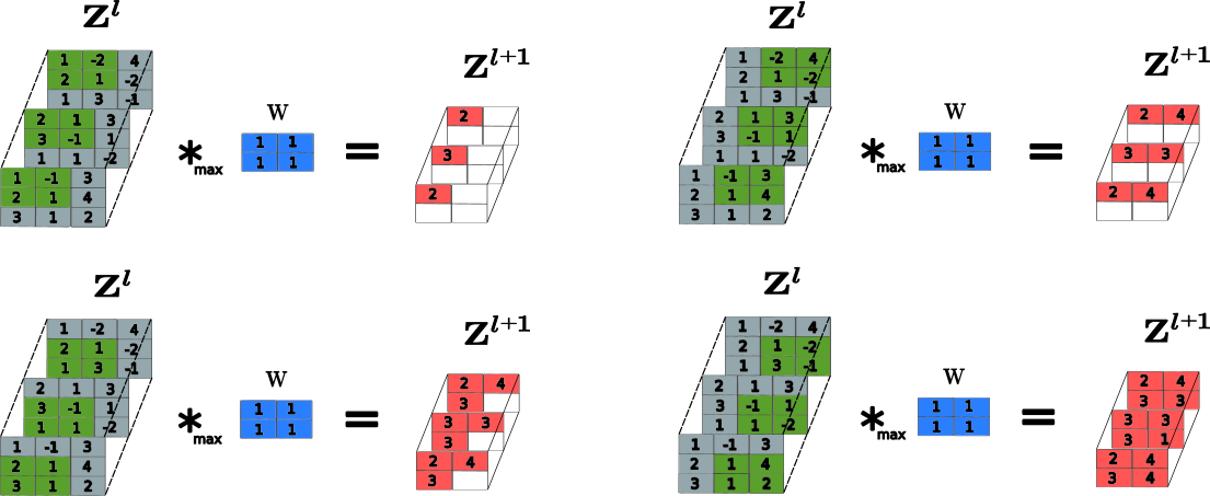
Consider a tensor $\mathbf{Z}^l$ with dimension $3 \times 3 \times 3$ ($n_l = 3$ and $m_l = 3$ channels) and window pool size $2 \times 2$. Applying the max pooling layer we will get the tensor $\mathbf{Z}^{l+1}$ of dimension $2 \times 2 \times 3$, as illustrated in the following image:
Convolutional Neural Network for Classification
Let’s create a classification model for the MNIST dataset to illustrate all the theory explained before. One possible approach for this classification model is to create two subclasses from the Model class: one for the convolutional and pooling layers, and another for the fully connected neural network layers. This modular design makes the customization easier for the CNN architecture to use with other kinds of input images.
We can alternate Conv2D layers with MaxPool2D layers. This arrangement enables the network to learn hierarchical features of increasing complexity and abstraction. It also reduces the spatial dimensionality of the feature maps, thereby improving the network’s computational efficiency.
Remember, the filter size in a Conv2D layer is a hyperparameter that determines the window size of the filter kernel as it slides over the input image matrix. Typically, the filter size is a small matrix, such as 3x3 or 5x5, which produces an output feature map that is passed to the next layer. In contrast, the pool size in a MaxPooling2D layer specifies the dimensions of the pooling window, which moves over the input feature map in two dimensions and outputs the maximum value of each window.
Now, let’s implement the classification model modularly using the Model class from tf.keras:
class CNN(Model):

    def __init__(self,
                 nn_model,
                 img_shape: tuple = (28, 28, 1),
                 filters: list = [32],
                 filter_size: list = [(3, 3)],
                 pool_sizes: list = [(2, 2)],
                 activation: str = 'relu',
                 filter_initializer: str = 'glorot_uniform') -> None:
        """
        Constructor for the CNN class.

        Parameters:
        nn_model (Model): An instance of a model that will receive the flattened features
        for final classification.
        img_shape (tuple): The shape of the input image.
        filters (list): A list specifying the number of filters in each convolutional layer.
        filter_size (list): A list specifying the dimensions of the filters in each convolutional layer.
        pool_sizes (list): A list specifying the dimensions of the pooling window for each maxpooling layer.
        activation (str): The activation function applied to each convolutional layer.
        filter_initializer (str): The initializer for the filters of the convolutional layers.
        """
        super(CNN, self).__init__()
        self.nn_model = nn_model
        self.img_shape = img_shape
        self.filters = filters
        self.filter_size = filter_size
        self.pool_sizes = pool_sizes
        self.activation = activation
        self.filter_initializer = filter_initializer

        # create convolutional layers
        self.conv2d = []
        for i in range(len(filters)):
            self.conv2d.append( Conv2D( filters = self.filters[i],
                                        kernel_size = self.filter_size[i],
                                        kernel_initializer = self.filter_initializer,
                                        input_shape = img_shape,
                                        activation = self.activation,
                                        name='Conv2D_{}'.format(i)))

        # create maxpooling layers
        self.maxpool = []
        for i in range(len(self.pool_sizes)):
            self.maxpool.append( MaxPool2D( pool_size=self.pool_sizes[i],
                                            name='MaxPool_{}'.format(i)))


        # create flatten layer to feed into the dense layer
        self.flatten = Flatten(name='Flatten')

    def call(self, x):
        """
        Forward pass of the network.

        Parameters:
        x (Tensor): The input tensor containing the image data.

        Returns:
        Tensor: The output tensor after applying the convolutional and pooling layers, and the final model.
        """
        for conv_layer, maxpool_layer in zip(self.conv2d, self.maxpool):
            x = conv_layer(x)
            x = maxpool_layer(x)
        x = self.flatten(x)
        x = self.nn_model(x)
        return x
class NN(Model):
    def __init__(
        self,
        layer_sizes: list = [128],
        output_size: int = 10,
        output_activation: str = "softmax",
        activation: str = "relu",
        weight_initializer: str = "glorot_uniform"
    ) -> None:
        """
        Constructor for the NN class.

        Parameters:
        layer_sizes (list): A list indicating the size of each dense layer.
        output_size (int): The number of units in the output layer.
        output_activation (str): The activation function for the output layer.
        activation (str): The activation function for all hidden layers.
        initializer (str): The initializer for the weights in all layers.
        """
        super(NN, self).__init__(name = 'Dense')

        self.layer_sizes = layer_sizes
        self.output_size = output_size
        self.activation_func = activation
        self.output_activation = output_activation
        self.weight_initializer = weight_initializer

        # Hidden Layers
        self.hidden_layer = []
        for i in range(len(layer_sizes)):
            self.hidden_layer.append(Dense( units = self.layer_sizes[i],
                                            kernel_initializer = self.weight_initializer,
                                            activation = activation,
                                            name='Dense_{}'.format(i)))

        # Output Layer
        self.output_layer = Dense( units= self.output_size,
                                    kernel_initializer = self.weight_initializer,
                                    activation=output_activation,
                                    name="Output" )

    def call(self, x: tf.Tensor) -> tf.Tensor:
        """
        Forward pass of the network, processing the input through
        each hidden layer followed by the output layer.

        Parameters:
        x (tf.Tensor): The input tensor.

        Returns:
        tf.Tensor: The resulting tensor after passing through all layers of the network.
        """
        for hidden in self.hidden_layer:
            x = hidden(x)
        x = self.output_layer(x)
        return x
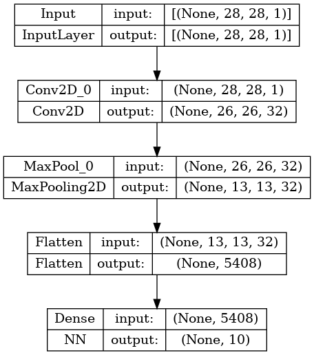
We can use the class Input as a placeholder to build a model and access its summary using the summary() method, as well as plot a diagram of the layers presented in this model:
x = Input(shape= (28,28,1), name="Input")
nn_model = NN()
cnn_model = CNN(nn_model)
summary_model = Model(inputs=x, outputs = cnn_model.call(x), name="CNN-Classification")

summary_model.summary()
Model: "CNN-Classification"
_________________________________________________________________
 Layer (type)                Output Shape              Param #
=================================================================
 Input (InputLayer)          [(None, 28, 28, 1)]       0

 Conv2D_0 (Conv2D)           (None, 26, 26, 32)        320

 MaxPool_0 (MaxPooling2D)    (None, 13, 13, 32)        0

 Flatten (Flatten)           (None, 5408)              0

 Dense (NN)                  (None, 10)                693642

=================================================================
Total params: 693962 (2.65 MB)
Trainable params: 693962 (2.65 MB)
Non-trainable params: 0 (0.00 Byte)
_________________________________________________________________
plot_model(summary_model, show_shapes=True, show_layer_names=True)
Let’s create a function to prepare and load our dataset with the digits from MNIST dataset:
def load_data():

    train = pd.read_csv('data/mnist_train_small.csv')
    test = pd.read_csv('data/mnist_test_small.csv')

    y_train = train['label'].to_numpy()
    x_train = train.drop('label', axis = 1).to_numpy()
    y_test = test['label'].to_numpy()
    x_test = test.drop('label', axis = 1).to_numpy()

    # reshape dataset to have a single channel
    # Reshape (20000,784) ->  (2000,     28,     28,     1)
    x_test = x_test.reshape(x_test.shape[0],28,28,1)
    x_train = x_train.reshape(x_train.shape[0],28,28,1)
    # one hot encode target values
    y_test = to_categorical(y_test)
    y_train = to_categorical(y_train)

    return (x_train, y_train, x_test, y_test)

def scale_pixels(train, test):
    # normalize the data to a range of [0, 1] and convert to float
    train_norm = train.astype('float32') / 255.0
    test_norm = test.astype('float32') / 255.0

    return train_norm, test_norm
# Data Pre-Processing
x_train, y_train, x_test, y_test = load_data()
x_train, x_test = scale_pixels(x_train, x_test)

# Model
nn_model = NN()
classification_model = CNN(nn_model)

# Compile and fit
classification_model.compile( loss = 'categorical_crossentropy',
                              optimizer = tf.optimizers.Adam(learning_rate=0.001),
                              metrics=['accuracy'])
classification_model.fit(x = x_train, y = y_train, epochs = 5, batch_size=32)
Epoch 1/5
625/625 [==============================] - 7s 11ms/step - loss: 0.2674 - accuracy: 0.9186
Epoch 2/5
625/625 [==============================] - 7s 11ms/step - loss: 0.0869 - accuracy: 0.9739
Epoch 3/5
625/625 [==============================] - 7s 11ms/step - loss: 0.0530 - accuracy: 0.9837
Epoch 4/5
625/625 [==============================] - 7s 11ms/step - loss: 0.0320 - accuracy: 0.9900
Epoch 5/5
625/625 [==============================] - 7s 11ms/step - loss: 0.0216 - accuracy: 0.9931


<keras.src.callbacks.History at 0x7f20a01cdae0>
def single_img(img_array):
"""
Reshape a single image array for prediction.
This function takes an image array, adds a batch dimension to it,
and returns the new array that is suitable for prediction with
models that expect batches of images.
Parameters:
img_array (np.array): The image array to be reshaped.
It should be a 2D array for a grayscale image.
Returns:
np.array: A new array with an added batch dimension.
"""
img_batch = np.expand_dims(img_array, axis=0)
return img_batch
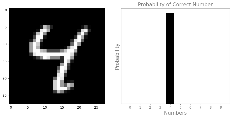
def plot_single_img(img, prediction, figsize=(10, 5)):
"""
Plot an image and its prediction probability distribution.
This function takes an image and a prediction array, and plots the image
and a bar chart representing the prediction probabilities for each class.
Parameters:
img (np.array): The image data to be plotted. It should be a 2D array.
prediction (np.array): The prediction data, where prediction[0] contains
the probability distribution across classes.
figsize (tuple): Optional. The size of the figure to be created.
Returns:
None: This function does not return a value but shows a matplotlib plot.
"""
fig, ax = plt.subplots(1, 2, figsize=figsize)
ax[0].imshow(img.reshape(28, 28), cmap='gray')
ax[1].bar(range(10), prediction[0], color='black')
ax[1].set_xlabel('Numbers', color="gray", fontsize=15)
ax[1].set_ylabel('Probability', color="gray", fontsize=15)
ax[1].set_title('Probability of Correct Number', color='gray', fontsize=15)
ax[1].set_xticks(range(10))
ax[1].set_yticks([])
ax[1].tick_params(axis='x', colors='gray', labelsize=10)
plt.tight_layout()
plt.show()
img_batch = single_img(x_test[6])
prediction = classification_model.predict(img_batch)
print(prediction)

plot_single_img(img_batch, prediction)
1/1 [==============================] - 0s 45ms/step
[[2.9586372e-11 1.2202437e-09 3.5340349e-11 9.1771851e-12 9.9999654e-01
  8.1947343e-10 3.6685540e-11 8.9030500e-08 3.1797342e-06 1.2824634e-07]]