Analysis of Diabetes Indicators

13 Dec 2023 - Tags: Classification, Random Forest, Decision Tree, and Logistic Regression

import pandas as pd
import numpy as np
import seaborn as sns
from matplotlib import pyplot as plt
from sklearn.model_selection import train_test_split, GridSearchCV, RandomizedSearchCV
from sklearn.metrics import auc, precision_score,recall_score ,roc_auc_score, confusion_matrix,\
                            f1_score, roc_curve
from sklearn.feature_extraction import DictVectorizer
from sklearn.tree import  DecisionTreeClassifier, plot_tree
from sklearn.ensemble import RandomForestClassifier
from sklearn.linear_model import LogisticRegression
from sklearn.feature_selection import mutual_info_classif
from sklearn.metrics import accuracy_score
from matplotlib.colors import ListedColormap

from scipy import stats
from scipy.stats import chi2_contingency
from sklearn.model_selection import GridSearchCV
from sklearn.preprocessing import StandardScaler, OneHotEncoder
from sklearn.compose import ColumnTransformer
from catboost import CatBoostClassifier, Pool

# Palette of colors used for the plots
red  = '#BE3232'
blue = '#2D4471' 

Outline

1. Data preparation
- 1.1. Split Dataset
2. Exploratory Data Analysis (EDA)
3. Model Training and Validation
4. Model Evaluation on Test Set
5. Conclusions

1. Data Preprocessing

The dataset used here is from kaggle. Let’s check the data:

df = pd.read_csv('../data/raw/diabete-indicators-balanced-5050split.csv')
display(df.head(2))

print("Before:",df.shape)
# Search for duplicated instances and drop
print("Duplications:",df.duplicated().sum())
#display(df.loc[df.duplicated(),:].head())
df.drop_duplicates(inplace=True)
print('After:',df.shape)

	Diabetes_binary	HighBP	HighChol	CholCheck	BMI	Smoker	Stroke	HeartDiseaseorAttack	PhysActivity	Fruits	...
0	0.0	1.0	0.0	1.0	26.0	0.0	0.0	0.0	1.0	0.0	...
1	0.0	1.0	1.0	1.0	26.0	1.0	1.0	0.0	0.0	1.0	...

2 rows × 22 columns

Before: (70692, 22)
Duplications: 1635
After: (69057, 22)

Let’s check if there are zeros in the categorical features where the range is above zero. This can be interpreted as missing values, so we need to change then to NaN.

categorical_columns = ["GenHlth", "MentHlth", "PhysHlth",
               "Age", "Education", "Income"]
for column in categorical_columns:
    print('Missing Values:', f'{round(100*df[column].eq(0).sum()/df.shape[0], 2)} %', f'in {column}')

print(f"Missing Values: {df['BMI'].eq(0).sum()} % in BMI")
df.drop(columns=['MentHlth', 'PhysHlth'], inplace=True)

categorical_columns = ["GenHlth", "MentHlth", "PhysHlth",
               "Age", "Education", "Income"]
for column in categorical_columns:
    print('Missing Values:', f'{round(100*df[column].eq(0).sum()/df.shape[0], 2)} %', f'in {column}')

print(f"Missing Values: {df['BMI'].eq(0).sum()} % in BMI")
df.drop(columns=['MentHlth', 'PhysHlth'], inplace=True)

There are indeed missing values for MentHlth and PhysHlth, both must have a range between 1-30. But because the missing values account for 67% of my dataset, it’s concerning. Even if this feature correlate highly with the target, removing 67% of data might be worse. A straightforward solution was just to drop these features.

1.1. Split Dataset

def convert_dtypes(df: pd.DataFrame, dtype_dict: dict) -> pd.DataFrame:
    """
    Convert the data types of specified columns for memory optimization.

    Parameters:
        df (pd.DataFrame): The original DataFrame.
        dtype_dict (dict): Dictionary specifying the columns and their corresponding data types.
                           Key: Desired data type (e.g., 'bool', 'int32', 'float32')
                           Value: List of columns to be converted to the key data type

    Returns:
        pd.DataFrame: DataFrame with optimized data types.
    """
    for dtype, columns in dtype_dict.items():
        for column in columns:
            df[column] = df[column].astype(dtype)
            

    return df

    # Before split, change the target name to Diabetes
df.rename(columns={'Diabetes_binary': 'Diabetes'}, inplace=True)

# Split in 60% Train /20% Validation/ 20% Test
df_train_large, df_test = train_test_split(df, test_size = 0.2, random_state = 1)
df_train, df_val = train_test_split(df_train_large, train_size = 0.75, random_state = 1)


# Save target feature
Y_train_large = df_train_large['Diabetes'].values
Y_test = df_test['Diabetes'].values
Y_train = df_train['Diabetes'].values
Y_val = df_val['Diabetes'].values

# Drop target feature 
df_train.drop('Diabetes', axis=1, inplace=True)
df_val.drop('Diabetes', axis=1, inplace=True)
df_test.drop('Diabetes', axis=1, inplace=True)

We will adjust the data types of df_train_large to optimize memory usage during the EDA process.

# for better memory usage and interpretability for EDA
boolean_columns = ['Diabetes',"HighBP", "HighChol", 
               "CholCheck", "Smoker", "Stroke", "HeartDiseaseorAttack",
               "PhysActivity", "Fruits", "Veggies", "HvyAlcoholConsump",  
               "AnyHealthcare", "NoDocbcCost", "DiffWalk", "Sex"]

categorical_columns = ["GenHlth", "Age", "Education", "Income"]

dtype_dict = {
    'int32': categorical_columns + boolean_columns,
    'float32': ["BMI"]
}

df_train_large = convert_dtypes(df_train_large, dtype_dict)
display(df_train_large.info())

<class 'pandas.core.frame.DataFrame'>
Index: 55245 entries, 15055 to 5239
Data columns (total 20 columns):
 #   Column                Non-Null Count  Dtype  
---  ------                --------------  -----  
 Diabetes              55245 non-null  int32  
 HighBP                55245 non-null  int32  
 HighChol              55245 non-null  int32  
 CholCheck             55245 non-null  int32  
 BMI                   55245 non-null  float32
 Smoker                55245 non-null  int32  
 Stroke                55245 non-null  int32  
 HeartDiseaseorAttack  55245 non-null  int32  
 PhysActivity          55245 non-null  int32  
 Fruits                55245 non-null  int32  
Veggies               55245 non-null  int32  
HvyAlcoholConsump     55245 non-null  int32  
AnyHealthcare         55245 non-null  int32  
NoDocbcCost           55245 non-null  int32  
GenHlth               55245 non-null  int32  
DiffWalk              55245 non-null  int32  
Sex                   55245 non-null  int32  
Age                   55245 non-null  int32  
Education             55245 non-null  int32  
Income                55245 non-null  int32  
dtypes: float32(1), int32(19)
memory usage: 4.6 MB

2. Exploratory Data Analysis (EDA)

Let’s proceed with the EDA in the df_train_large dataset, which is the combination of both training and validation sets. To prevent data leakage, we don’t include the test set for the EDA. This will ensure the trained model evaluation on the test set is unbiased, without information from the train set mistakenly leakage to the test.

2.1 Feature Distribution

# Create a dataset without the target feature
df_train_dropped = df_train_large.drop('Diabetes', axis=1)

features = df_train_dropped.columns
n_features = len(features)

fig, axes = plt.subplots(nrows = 7, ncols=3, figsize=(15, 15))

for idx, feature in enumerate(features):
    # Identify row and column in the grid
    row, col = divmod(idx, 3)
    
    # Check if the feature is boolean type
    if np.issubdtype(df_train_dropped[feature].dtype, np.bool_):
        Yes_count = np.sum(df_train_large[feature])
        No_count = len(df_train_large[feature]) - Yes_count
        axes[row, col].bar(['Yes', 'No'], [Yes_count, No_count], color=blue, alpha = 0.4)
    else:
        # Plot histogram for the current feature
        axes[row, col].hist(df_train_dropped[feature], bins=50, color=blue, alpha = 0.8,)

    axes[row, col].set_title(feature)
    axes[row, col].grid(axis='y')

# remove empty plots
for ax in axes.ravel()[len(features):]:
    ax.axis('off')

# Adjust layout
plt.tight_layout()
plt.show()

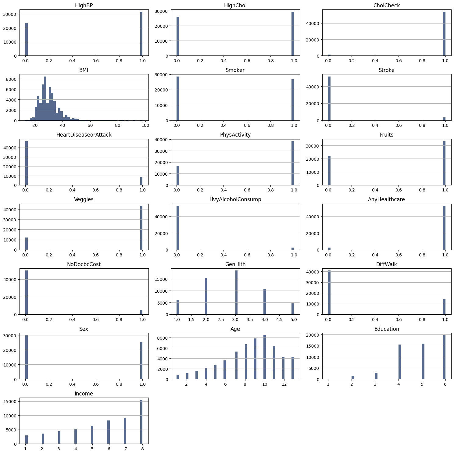
Most of our features are categorical. Features like CholCHeck, Stroke, HeartDiseaseorAttack, Vaggies, HvyAlcoholConsump, AnyHealthcare, NoDocbcCost are highly concentrated in one category. This suggests that there may be a common characteristic shared among most individuals for each of these features, resulting in skewed distributions. While this skewness in feature distribution does not present the same challenges as an imbalanced target, it may still impact the interpretability and performance of our predictive models, particularly if these features are strongly associated with the target.

Also, it’s appear that the feature BMI has outliers that wee need to take a closer look.

# From World Health Organization (WHO):
#---------------------------
# Under: BMI less than 18.5
# Normal: BMI between 18.5 and 24.9
# Over: BMI between 25 and 29.9
# Obesity: BMI of 30 or greater

fig, axes = plt.subplots(1, 2, figsize=(10, 5))

# Plot the histplot on the first axes
sns.histplot(df_train_dropped['BMI'], bins=50, alpha=0.4, color=blue, ax=axes[0])

# Add vertical lines
for line in [18.5, 24.9, 29.9]:
    axes[0].axvline(line, color= red, linestyle='--', alpha=0.5)

# Add text labels within the second subplot (histplot)
categories = ['Under', 'Normal', 'Over', 'Obesity']
positions = [12, 21.7, 27.45, 50]  # Midpoints between the lines and the ends

for x_pos, cat in zip(positions, categories):
    axes[0].text(x_pos, 5500, cat, rotation=90, size=10, va='bottom')

axes[0].set_title('BMI Histogram')

#-------
# Plot the boxplot on the second axes
sns.boxplot(data=df_train_dropped, y='BMI', color=blue, width=0.5, fliersize=3, ax=axes[1])
axes[1].set_title('BMI Boxplot')

# Add horizontal lines
for line in [18.5, 24.9, 29.9]:
    axes[1].axhline(line, color= red, linestyle='--', alpha=0.5)


# Display the plots
plt.tight_layout()
plt.show()

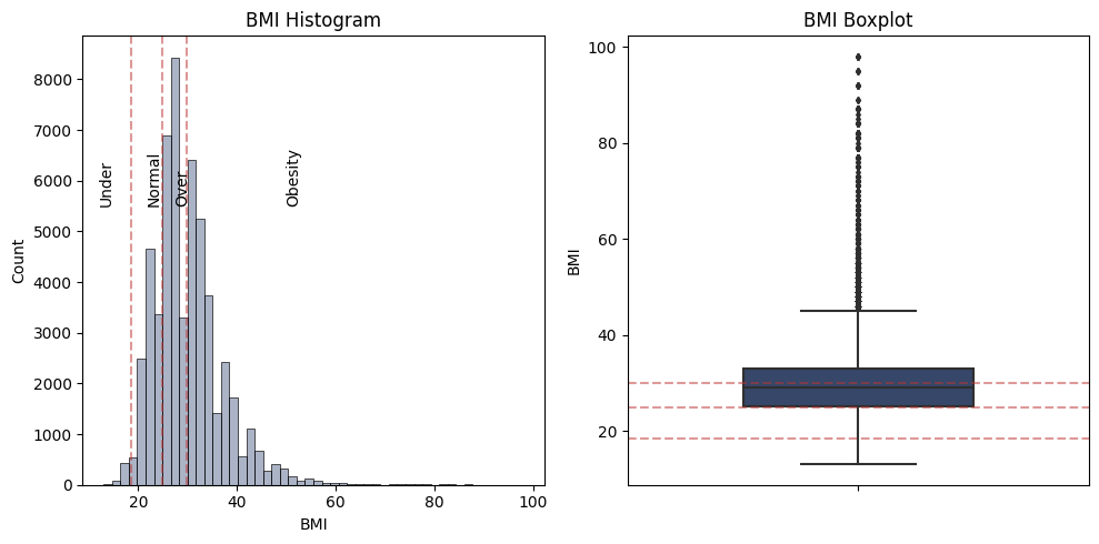
There are numerous outliers, indicating individuals with significantly higher BMI values. Given the skewed distribution and box plot, these outliers do not necessarily represent errors or anomalies in the data but rather a realistic representation of the upper bound of BMI within the population.

2.2 Feature Importance

def plot_feature_importance(df, x, y, ax, threshold=0.002, pad=5.0, title='Feature Importance', 
                            xlabel='Features', ylabel='Importance', palette=None):
    """
    Function to plot the feature importance with a distinction of importance based on a threshold.

    Parameters:
    - df: pandas.DataFrame
        DataFrame containing features and their importance scores.
    - x: str
        Name of the column representing feature names.
    - y: str
        Name of the column representing feature importance scores.
    - ax: matplotlib axis object
        Axis on which to draw the plot.
    - threshold: float, optional (default=0.002)
        Value above which bars will be colored differently.
    - pad: float, optional (default=5.0)
        Adjust the layout of the plot.
    - title: str, optional (default='Feature Importance')
        Title of the plot.
    - xlabel: str, optional (default='Features')
        Label for the x-axis.
    - ylabel: str, optional (default='Importance')
        Label for the y-axis.
    - palette: list, optional
        A list of two colors. The first color is for bars below the threshold and the second
        is for bars above.

    Returns:
    - None (modifies ax in-place)
    """
    if palette is None:
        palette = ["blue", "red"]
    
    blue, red = palette
    colors = [red if value >= threshold else blue for value in df[y]]
    sns.barplot(x=x, y=y, data=df, ax=ax, alpha=0.5, palette=colors)
    ax.set_xticklabels(df[x], rotation=70, fontsize=12)
    ax.set_ylabel(ylabel, fontsize=15)
    ax.set_xlabel(xlabel, fontsize=15) 
    ax.grid(axis='y')
    ax.set_title(title, fontsize=15)
    plt.tight_layout(pad=pad)

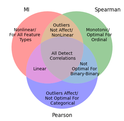
Mutual Information

Given that most of our features are binary, having only one numerical feature for BMI, a first natural choice of metric to account correlation would be the Mutual information (MI). MI accounts for linear and non-linear relation, is robust against outliers and can be reliable for any numerical or categorical features.

Let’s compare the MI of the features with the target variable Diabetes.

mi_values = mutual_info_classif(df_train_dropped, Y_train_large, discrete_features=True)

mi_column = pd.DataFrame(mi_values, index=pd.Index(df_train_dropped.columns, name='features'), 
                         columns=['diabetes_MI']).sort_values(by='diabetes_MI', ascending=False)

# Convert the index 'Features' into a column for plotting
mi_column_reset = mi_column.reset_index()

# Plotting
feature_threshold= 0.020
fig, ax = plt.subplots(figsize=(15, 10))
plot_feature_importance(mi_column_reset, x='features', y='diabetes_MI', ax=ax, threshold=feature_threshold, 
                        title="Mutual Information With Diabetes", xlabel="Features", 
                        ylabel="Diabetes MI", palette=[blue, red])

plt.show()

# Select features with MI > feature_threshold
best_mi_features = list(mi_column[mi_column['diabetes_MI'] > feature_threshold].index)
print("Best correlated features:\n",best_mi_features)

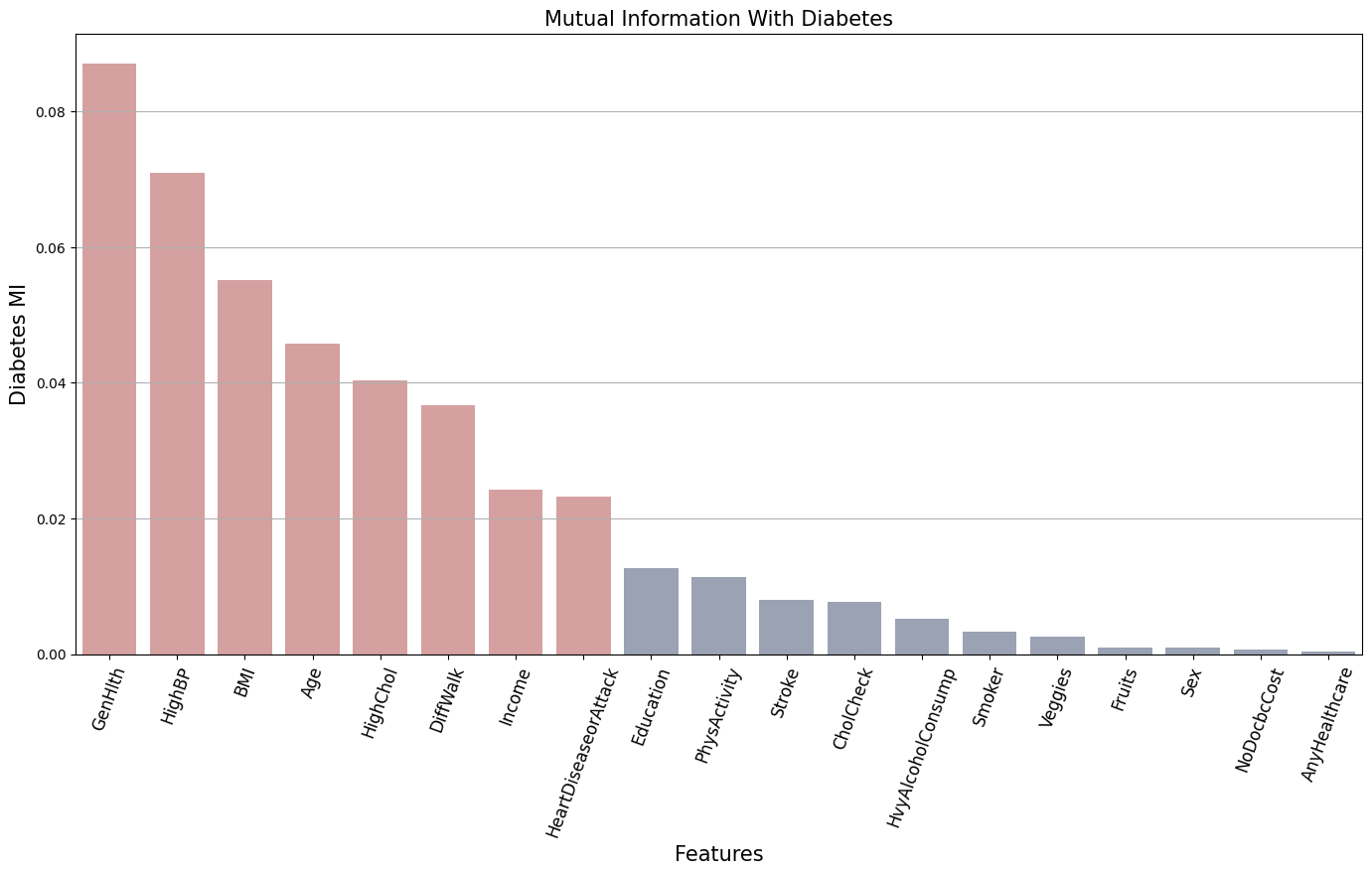
Best correlated features:
 ['GenHlth', 'HighBP', 'BMI', 'Age', 'HighChol', 'DiffWalk', 'Income', 'HeartDiseaseorAttack']

The bars in red represent the features related to the target variable Diabetes that preset the most significant entropy reduction. This means that these features provide significant information about the presence of diabetes.

Spearman Correlation

Some of our features, like GenHlth, MentHlth, PhysHlth, `Age, Education, Income are ordinal. A useful metric for this case is Spearman Correlation. Spearman Correlation is a non-parametric metric (does not assume any specific distribution for the data) and are more reliable to ordinal data. It captures monotonic relationships, whether linear or not.

Let’s compare the Spearman Correlation of the features with the target variable Diabetes.

# Calculate Spearman correlation
spearman_corr = df_train_large.corr(method='spearman')['Diabetes'].agg(np.abs)\
                                                .sort_values(ascending=False)\
                                                .drop('Diabetes')\
                                                .to_frame()

# Convert Spearman correlation to DataFrame and reset index
spearman_column = spearman_corr.reset_index()
spearman_column.columns = ['Features', 'spearman_correlation']

# Plotting
feature_threshold= 0.07
fig, ax = plt.subplots(figsize=(15, 10))
plot_feature_importance(spearman_column, x='Features', y='spearman_correlation', ax=ax, 
                        threshold=feature_threshold, 
                        title="Spearman Correlation With Diabetes", xlabel="Features", 
                        ylabel="Diabetes Correlation", palette=[blue, red])

plt.show()

# Select features with Spearman correlation value > feature_threshold
best_spearman_features = spearman_corr[spearman_corr['Diabetes'] >= feature_threshold].index.tolist()
print("Best correlated features:\n", best_spearman_features)

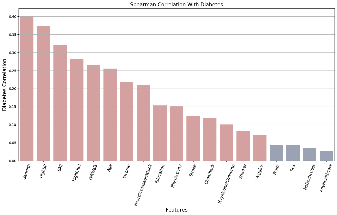
Best correlated features:
 ['GenHlth', 'HighBP', 'BMI', 'HighChol', 'DiffWalk', 'Age', 'Income', 'HeartDiseaseorAttack', 
 'Education', 'PhysActivity', 'Stroke', 'CholCheck', 'HvyAlcoholConsump', 'Smoker', 'Veggies']

Let’s check one more metric, Pearson correlation. While Spearman detects monotonic relationships, Pearson captures linear relationships.

Pearson Correlation

The Pearson correlation accounts only for linear relationships and is very sensitive to outliers. It’s not particularly reliable for categorical data, especially binary ones.

# Calculate Spearman correlation
pearson_corr = df_train_large.corr(method='pearson')['Diabetes'].agg(np.abs)\
                                                .sort_values(ascending=False)\
                                                .drop('Diabetes')\
                                                .to_frame()

# Convert Spearman correlation to DataFrame and reset index
pearson_column = pearson_corr.reset_index()
pearson_column.columns = ['Features', 'pearson_correlation']

# 
feature_threshold = 0.07
fig, ax = plt.subplots(figsize=(15, 10))
plot_feature_importance(pearson_column, x='Features', y='pearson_correlation', ax=ax, 
                        threshold=feature_threshold, 
                        title="Pearson Correlation With Diabetes", xlabel="Features", 
                        ylabel="Diabetes Correlation", palette=[blue, red])

plt.show()


# Select features with correlation value > feature_threshold
best_pearson_features = pearson_corr[pearson_corr['Diabetes'] >= feature_threshold].index.tolist()
print("Best correlated features:\n", best_pearson_features)

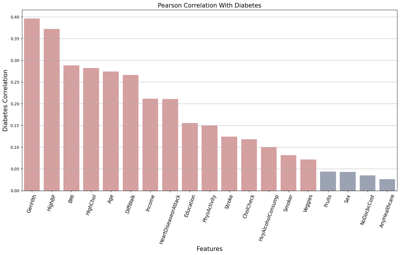
Best correlated features:
 ['GenHlth', 'HighBP', 'BMI', 'HighChol', 'Age', 'DiffWalk', 'Income', 'HeartDiseaseorAttack', 
 'Education', 'PhysActivity', 'Stroke', 'CholCheck', 'HvyAlcoholConsump', 'Smoker', 'Veggies']

Utilizing three distinct metrics — Mutual Information (MI), Pearson, and Spearman — I constructed a schematic representation of a diagram that illustrates the shared and unique characteristics of each metric.

The diagram can provide a better view of how these metrics intersect and which features emerge as a relevant correlation with the target variable.

Using this idea, let take the overlapping sets of features selected by each metric.

mi_set = set(best_mi_features)
pearson_set = set(best_pearson_features)
spearman_set = set(best_spearman_features)

# Common features across pearson and mutual information
pearson_mi_set = (pearson_set.intersection(mi_set))
print("\n Pearson and MI intersection:\n",pearson_mi_set)

# Common features across spearman and mutual information
spearman_mi_set = (spearman_set.intersection(mi_set))
print("\n Spearman and MI intersection:\n",spearman_mi_set)

# Common features across spearman and pearson
spearman_pearson_set = (spearman_set.intersection(pearson_set))
print("\n Spearman and Pearson intersection:\n",spearman_pearson_set)

# Common features across all three metrics
small_feature_set = mi_set.intersection(pearson_set).intersection(spearman_set)
print("\nIntersection for all metrics:\n",small_feature_set)

 Pearson and MI intersection:
 {'BMI', 'HighBP', 'HighChol', 'Income', 'DiffWalk', 'HeartDiseaseorAttack', 'GenHlth', 'Age'}

 Spearman and MI intersection:
 {'BMI', 'HighBP', 'HighChol', 'Income', 'DiffWalk', 'HeartDiseaseorAttack', 'GenHlth', 'Age'}

 Spearman and Pearson intersection:
 {'HvyAlcoholConsump', 'BMI', 'PhysActivity', 'HighBP', 'CholCheck', 'HighChol', 'Income', 
 'DiffWalk', 'HeartDiseaseorAttack', 'GenHlth', 'Age', 'Education', 'Stroke', 'Veggies', 'Smoker'}

Intersection for all metrics:
 {'BMI', 'HighBP', 'HighChol', 'Income', 'DiffWalk', 'HeartDiseaseorAttack', 'GenHlth', 'Age'}

From this analyze for the correlations we can conclude that the features BMI, GenHlth, Age, Income, HeartDiseaseorAttack, DiffWalk, HighBP, HighChol appear to have a higher degree of relevance compare to the target Diabetes. All three metrics show a agreement for the relevance of these features.

Now, with a more restricted set of features, it’s essential to closely examine the relationship between the each feature and the target variable based on their frequency. To do this, we can create a frequency table and illustrate the results using a bar plot.

Let’s take the set with the common feature across all three metrics to proceed with the analyze.

# Separate in binary and non binary
numerical = ['BMI']
categorical = ['GenHlth', 'Age', 'Income']
binary = ['HighChol','DiffWalk', 'HighBP', 'HeartDiseaseorAttack']

Binary

fig, axes = plt.subplots(2, 2, figsize=(17, 10))

for ax, feature in zip(axes.ravel(), binary):

    ct = pd.crosstab(df_train_dropped[feature], Y_train_large )
    ct_normalized = ct.divide(ct.sum(axis=0), axis=1)*100

    ct_normalized.plot(kind='bar', stacked=False, ax=ax, color = [blue, red],
             alpha = 0.5, fontsize= 15, legend=False  )
    #sns.barplot(x=ct_normalized.index, y= ct_normalized[1], ax=ax, palette = ['#2D4471', '#BE3232'], alpha = 0.5)
    
    ax.set_title('', fontsize=21)
    ax.set_ylabel('Percentage %', fontsize= 18)
    ax.set_xlabel(feature, fontsize= 18)

    ax.set_xticks([0, 1])  
    ax.set_xticklabels(['No', 'Yes'], fontsize=18, rotation=45)
    ax.legend( ['No Diabetes', 'Diabetes'], title=' ', 
               loc='upper center', fontsize = 14)

#for ax in axes.ravel()[len(binary):]:
#    ax.axis('off')

plt.tight_layout(pad=5.0)
plt.show()

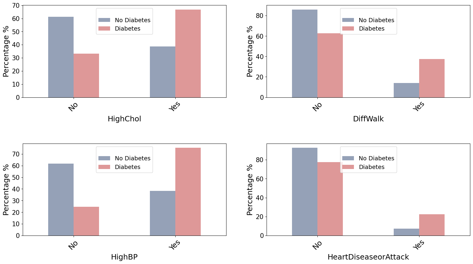
For Binary (categorical) data we can use the chi squared test to quantify how independent two categorical variables are, i.e. if there is an association between the two variables. This is achieved by this statistical test by comparing the observed frequencies to expected frequencies in a contingency table for the classes.

cts = {}
for feature in binary:
    # Compute the contingency table
    ct = pd.crosstab(df_train_dropped[feature], Y_train_large)    
    cts[feature] = ct 
    # chi-squared test
    _, p_value, _, _ = chi2_contingency(cts[feature])

    # Null hypothesis: There is no association between the two variables
    if (p_value < 0.05):
        print(f"Significant association between diabetes status and {feature}.")

    else:
        print('Failed to reject Null Hypothesis')

Significant association between diabetes status and HighChol.
Significant association between diabetes status and DiffWalk.
Significant association between diabetes status and HighBP.
Significant association between diabetes status and HeartDiseaseorAttack.

The visualization in a bar plot for HighChol, DiffWalk, HighBP demonstrates a tendency to Diabetes when the answer is Yes. The visual observation is further supported by the chi-squared test. Thus, it can be inferred that Diabetic patients tend to have higher cholesterol, difficulty walking, and higher blood pressure.

On the other hand, while HeartDiseaseorAttack seems to have an association with Diabetes, this link is less evident in the visual observation.

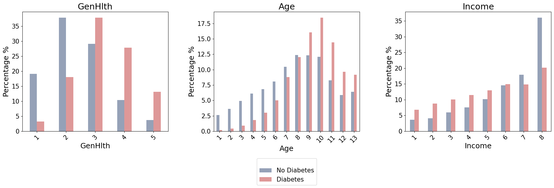
Categorical Ordinal

fig, axes = plt.subplots(1, len(categorical), figsize=(20, 8))

for ax, feature in zip(axes.ravel(), categorical):

    ct = pd.crosstab(df_train_dropped[feature], Y_train_large)
    ct_normalized = ct.divide(ct.sum(axis=0), axis=1)*100

    ct_normalized.plot(kind='bar', stacked=False, ax=ax, color=[blue, red], 
            alpha=0.5, fontsize=15, legend=False)

    ax.set_title(feature, fontsize=21)
    ax.set_ylabel('Percentage %', fontsize=18)
    ax.set_xlabel(feature, fontsize=18)

    # Allow x-axis tick labels to take on unique values for non-binary variables
    ax.tick_params(axis='x', rotation=45, labelsize=15)
    
axes[1].legend(['No Diabetes', 'Diabetes'], title=' ', loc='upper center', 
              bbox_to_anchor=(0.5, -0.2), fontsize=15)

#for ax in axes.ravel()[len(non_binary):]:
#    ax.axis('off')

plt.tight_layout(pad=5.0)
plt.show()

cts = {}
for feature in categorical:
    # Compute the contingency table
    ct = pd.crosstab(df_train_dropped[feature], Y_train_large)    
    cts[feature] = ct 
    # chi-squared test
    _, p_value, _, _ = chi2_contingency(cts[feature])

    # Null hypothesis: There is no association between the two variables
    if (p_value < 0.05):
        print(f"Significant association between diabetes status and {feature}.")

    else:
        print('Failed to reject Null Hypothesis')

Significant association between diabetes status and GenHlth.
Significant association between diabetes status and Age.
Significant association between diabetes status and Income.

For GenHlth it shows a correlation with diabetes. Based on the categories of general health:

excellent : less than $5\%$ has diabetes
very good : between $15-20 \%$ has diabetes
good: more than $35\%$ has diabetes
fair: between $25-30 \%$ has diabetes
poor: between $10-15 \%$ has diabetes

As general health gets worse, the percentage of individuals diagnosed with diabetes increases.

For the Age we have the following categories:

18-24
25-29
30-34
35-39
40-44
45-49
50-54
55-59
60-64
65-69
70-74
75-79
more then 80

There’s an observed increment in the percentage of individuals with diabetes as age progresses, though there are some exceptions. This is a good sign, because it is in line with known medical data indicating that the risk of diabetes increases with age.

For Income , those individuals with the highest income tend to have an increase in the incidence of diabetes compared to lowest income. But is complex to say more than this, because it does not follow a simple linear trend as for GenHlth and Age.

Numerical

# Divide the dataset into two groups based on Diabetes status
df_train_no = df_train_large[df_train_large['Diabetes'] == 0]
df__train_yes = df_train_large[df_train_large['Diabetes'] == 1]

# Select the BMI feature from each group
df_no_bmi = df_train_no['BMI']
df_yes_bmi = df__train_yes['BMI']


fig, axes = plt.subplots(nrows=1, ncols=2, figsize=(14, 6))

# Plotting the distributions
sns.kdeplot(df_yes_bmi, ax=axes[0],color=red , alpha=0.4, fill=True)
sns.kdeplot(df_no_bmi, ax=axes[0],color=blue , alpha=0.4, fill=True)

axes[0].axvline(df_yes_bmi.mean(), color=red, linestyle='--', alpha = 1)
axes[0].axvline(df_no_bmi.mean(), color=blue, linestyle='--', alpha = 1)

axes[0].text(df_yes_bmi.mean(), -0.007, f'{df_yes_bmi.mean():.1f}',
              color=red, rotation=90, ha='center')

axes[0].text(df_no_bmi.mean(), -0.007, f'{df_no_bmi.mean():.1f}',
              color=blue, rotation=90, ha='center')



axes[0].grid()
axes[0].set_title('BMI Distribution')
axes[0].legend(['Diabetics', 'No-diabetes'])

# Plotting the CDFs
sns.ecdfplot(df_yes_bmi, ax=axes[1], label="Diabetics", 
             color=red, alpha=0.6)

sns.ecdfplot(df_no_bmi, ax=axes[1], label="No-diabetes", 
             color=blue, alpha=0.6)

axes[1].grid()
axes[1].set_title('BMI Cumulative Distribution')
axes[1].legend()

plt.tight_layout(pad=5.0)
plt.show()

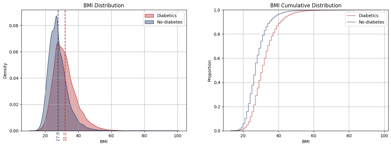
For numerical data, we employ the t-test to compare the means of two groups: BMI for diabetic patients and BMI for non-diabetic patients. Because the variances of the groups differ, then Welch’s t-test is employed, not assuming equal variances.

print('Diff of Variances:', np.abs(df_yes_bmi.var() - df_no_bmi.var()))
# the variance of the two groups are different, so we use Welch's t-test
_, p_value  = stats.ttest_ind(df_yes_bmi, df_no_bmi, equal_var=False)

# Null hypothesis: The two groups have the same mean
if p_value < 0.05:   
    print('Diabetic and non-diabetic have different BMI')
else:
    print('Failed to reject Null Hypothesis')

Diff of Variances: 16.09348
Diabetic and non-diabetic have different BMI

The distributions and cumulative distribution for BMI in diabetic and non-diabetic patients has a significant difference. The BMI distribution for diabetics appears right-skewed, suggesting a tendency towards higher BMI values compared to the more symmetric distribution of non-diabetics. This difference is more evident in their cumulative distributions, which show a significant gap between the curves. This visual observation is further supported by a Welch’s t-test, indicating a significant difference in the mean BMI values of the two groups. Thus, it can be inferred that diabetic patients tend to have higher BMIs than non-diabetics

2.3 Conclusion from EDA

After analyzing the data, we found that the best features for training our machine learning model are:

HighBP
GenHlth
HighChol
DiffWalk
Age
BMI
HeartDiseaseorAttack
Income

We saw a clear link between these features and the target variable Diabetes. But for the HeartDiseaseorAttack and Income features, it’s harder to say exactly how they relate or if the relationship is significant for predicting whether an individual has diabetes. All we can infer is that the relationship is not linear. Also, HeartDiseaseorAttack is highly centred in one category, and this could have some influence in this relation with the target variable.

3. Model Training and Validation

Now, with a better understanding of the features and their significance in relation to the target variable Diabetes, we can proceed to train a model to evaluate its performance on this set of features identified from the EDA. We consider both a consensus set of features, where all metrics agree, which results in a smaller feature set, and a large set of features selected based on the highest Pearson and mutual information. This approach will allow us to compare the models using different subsets of features, providing a more nuanced understanding of the relevance (or irrelevance) of each feature to the target variable.

# Remove Diabetes, is not necessary anymore
boolean_features = boolean_columns.copy()
boolean_features.remove('Diabetes')
categorical_features  = categorical_columns.copy()

# Best set of features selected from EDA
small_feature_list = list(small_feature_set)

large_feature_set = spearman_pearson_set.union(mi_set)
large_feature_list= list(large_feature_set)

def categorical_encoding(df_train , df_val , df_test ,features = None , sparse = False ):
    """
    Function to preprocess data frames based on the selected features.
    
    Parameters:
    - df_train, df_val, df_test: pandas.DataFrame or None
        Training, validation, and test datasets.
    - features: list
        List of features to be selected from the data frames.
        
    Returns:
    - X_train, X_val_small, X_test_small: numpy.ndarray or None
        Processed feature arrays for training, validation, and test datasets.
    - dv: DictVectorizer
        Fitted DictVectorizer object.
    """
    
    if features is None:
        features = df_train.columns.tolist()
    else:
        df_train = df_train[features].copy()
        df_test = df_test[features].copy()
        df_val = df_val[features].copy()
    
    dv = DictVectorizer(sparse= sparse)
    dataframes = {'train': df_train, 'val': df_val, 'test': df_test}
    transformed_data = {}
    fitted = False
    
    for key, df in dataframes.items():
            
        df_dict = df.to_dict(orient='records')
        if not fitted:
            transformed_data[key] = dv.fit_transform(df_dict)
            fitted = True 
        else:
            transformed_data[key] = dv.transform(df_dict)

    return transformed_data.get('train'), transformed_data.get('val'), transformed_data.get('test'), dv

def model_train_preprocess(df_train, df_val, df_test, selected_features_eda : list,  
                           featurers_to_dtype: dict = None, features_to_scale: list =None):
    
    dfs = [df_train, df_val, df_test]
    
    # Standardize features_to_scale if provided
    if features_to_scale:
        scaler = StandardScaler()
        scaler.fit(df_train[features_to_scale])
        for df in dfs:
            df[features_to_scale] = scaler.transform(df[features_to_scale])
    
    # Convert data types if dtype_dict is provided
    if featurers_to_dtype:
        for df in dfs:
            df = convert_dtypes(df, featurers_to_dtype)

    # Encode categorical variables for selected features from EDA
    return categorical_encoding(df_train, df_val, df_test, selected_features_eda)

3.1 Logistic Regression

# Best set of features selected from EDA
small_feature_list = list(small_feature_set)
large_feature_list= list(spearman_pearson_set.union(mi_set))

print('\n Small set of features:\n', small_feature_list)
print('\n Large set of features:\n', large_feature_list)

# Change dtypes for logistic regression
dtype_dict_lr = {
    'bool': boolean_features,
    'str': categorical_features,
    'float32': ["BMI"]
}

# Create a copy of dataframe to modify the dtypes
df_train_lr = df_train.copy()
df_val_lr = df_val.copy()
df_test_lr = df_test.copy()

X_train_small, X_val_small, _, _ = model_train_preprocess( df_train_lr, df_val_lr, df_test_lr, 
                                                           small_feature_list,
                                                           dtype_dict_lr, features_to_scale=['BMI'])

X_train_large, X_val_large, _, _ = model_train_preprocess( df_train_lr, df_val_lr, df_test_lr, 
                                                           large_feature_list,
                                                           dtype_dict_lr, features_to_scale=['BMI'])

Small set of features:
['BMI', 'HighBP', 'HighChol', 'Income', 'DiffWalk', 'HeartDiseaseorAttack', 'GenHlth', 'Age']

Large set of features:
['HvyAlcoholConsump', 'BMI', 'HighChol', 'DiffWalk', 'HeartDiseaseorAttack', 'GenHlth', 
'Age', 'Veggies', 'PhysActivity', 'HighBP', 'CholCheck', 'Income', 'Stroke', 'Education', 'Smoker']

3.1.1 Hyperparameter tunning and validate

# Grid search cross validation
grid={"C":[0.001, 0.01, 1, 10, 100],
      "penalty":["l1","l2"],
      "solver": [ 'liblinear']}

lr_model =LogisticRegression(random_state = 42)
lr_model_cv=GridSearchCV(lr_model, grid, cv=10)
lr_model_cv.fit(X_train_large, Y_train)

print("Tuned hyperparameters :",lr_model_cv.best_params_)
print("Accuracy of the best hyperparameters :",round(lr_model_cv.best_score_,3))

Y_pred_lr_large = lr_model_cv.best_estimator_.predict(X_val_large)
print('\n Accuracy for Large Feature Set:', round(accuracy_score(Y_pred_lr_large, Y_val), 3))

# 'C': 1, 'penalty': 'l2', 'solver': 'liblinear'

Tuned hyperparameters : {'C': 1, 'penalty': 'l2', 'solver': 'liblinear'}

Accuracy of the best hyperparameters : 0.744

Accuracy for Large Feature Set: 0.748

# Train and validate baseline features
lr_model= LogisticRegression(solver='liblinear', penalty= 'l2', C = 1, random_state=1)
lr_model.fit(X_train_small, Y_train)
Y_pred_lr_small = lr_model.predict(X_val_small)


print('Accuracy for Small Feature Set:',round(accuracy_score(Y_pred_lr_small, Y_val), 3))

Accuracy for Small Feature Set: 0.744

3.1.2 Feature importance

def feature_elimination(df_train, df_val, Y_train, Y_val, model, metric_func, features, base_metric):
    """
    Function to perform feature elimination based on the given model and metric function.

    Parameters:
    - df_train, df_val: pandas.DataFrame
        Training and validation datasets.
    - Y_train, Y_val: pandas.Series or numpy.ndarray
        Target values for training and validation datasets.
    - model: scikit-learn estimator
        The machine learning model to be trained.
    - metric_func: callable
        The metric function to evaluate model performance.
    - base_metric: float
        The base accuracy or metric value to compare against.

    Returns:
    - df_feature_metrics: pandas.DataFrame
        DataFrame showing the impact of each feature's elimination on model performance.
    """
    
    eliminated_features = []
    metric_list = []
    metric_diff_list = []   # to store the difference
    metric_name = metric_func.__name__

    for feature in features:

        df_train_drop = df_train.drop(feature, axis=1, inplace=False)
        df_val_drop = df_val.drop(feature, axis=1, inplace=False)
        X_train_small, X_val_small, _, _ = categorical_encoding(df_train_drop, df_val_drop, df_val_drop)

        model.fit(X_train_small, Y_train)
        Y_pred = model.predict(X_val_small)
        metric_score = metric_func(Y_pred, Y_val)
        
        # Store results in lists
        eliminated_features.append(feature)
        metric_list.append(metric_score)
        metric_diff_list.append(abs(base_metric - metric_score))  # compute the difference

    df_feature_metrics = pd.DataFrame({ 
        'eliminated_feature': eliminated_features,
        f'{metric_name}': metric_list,
        f'{metric_name}_diff': metric_diff_list  # add the difference as a column
    })\
    .sort_values(by=[f'{metric_name}_diff'], ascending=False)

    return df_feature_metrics

lr_model = LogisticRegression(solver='liblinear',  penalty= 'l1', C = 1, random_state = 42)
feature_importance = feature_elimination(df_train, df_val, Y_train, Y_val,
                                   lr_model, accuracy_score, large_feature_list, 
                                   accuracy_score(Y_pred_lr_large, Y_val) )

#display(feature_importance)


fig, ax = plt.subplots(figsize=(15, 8))

importance_threshold = 0.005
colors = [red if value >= importance_threshold else blue for value in feature_importance['accuracy_score_diff']]
sns.barplot(x="eliminated_feature", y="accuracy_score_diff", 
            data=feature_importance, ax=ax, alpha=0.5, palette=colors)

ax.set_xticklabels(feature_importance["eliminated_feature"], rotation=45, fontsize=12)
ax.set_ylabel('Accuracy Difference (Importance)', fontsize=15)
ax.set_xlabel('Features', fontsize=15) 
ax.grid(axis='y')
ax.set_title('Feature Elimination ', fontsize=15)
plt.tight_layout(pad=5.0)
plt.show()

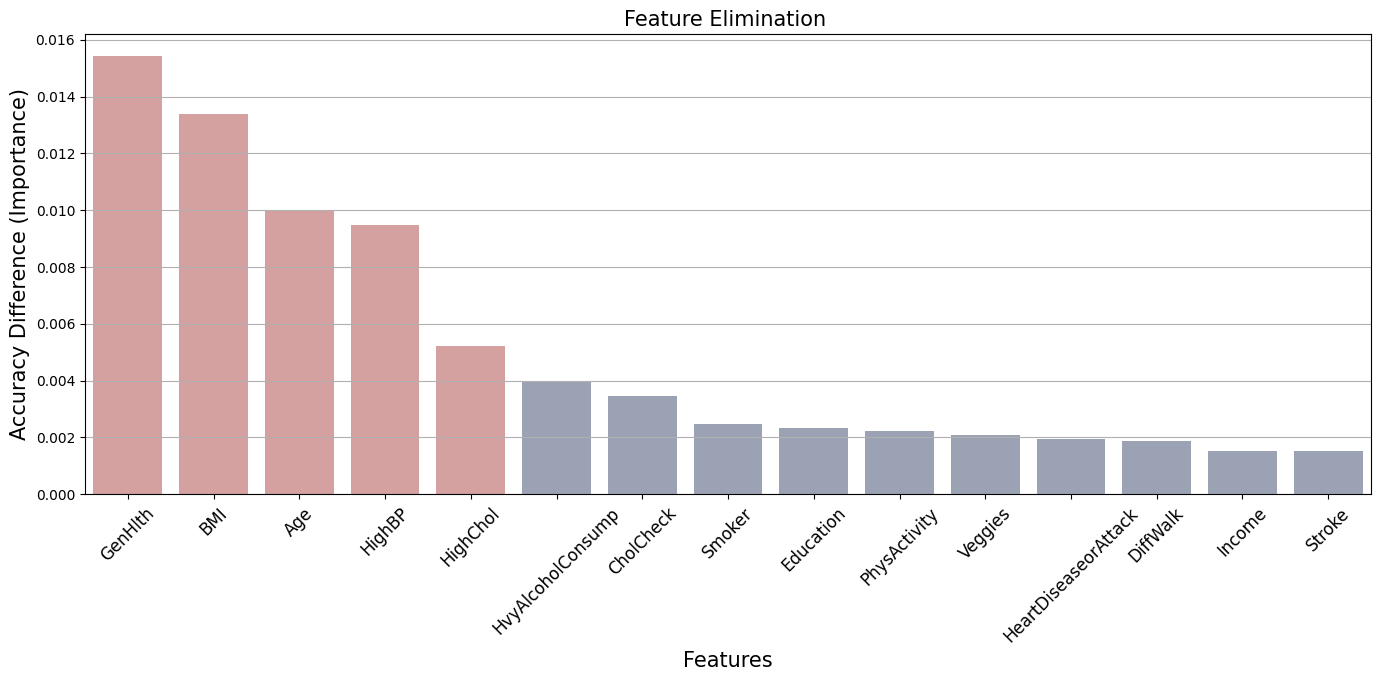
The table indicates that the features GenHlth, BMI, Age, HighBP, HighChol are relevant for the model’s accuracy. Removing any of these specific features leads to a large decline in accuracy compared to the others features.

# Save most important features for logistic regression
feature_importance_lr = set(
  feature_importance[feature_importance['accuracy_score_diff'] >= importance_threshold]['eliminated_feature']
    )
print('\nFeatures importance Logistic Regression:\n', feature_importance_lr)

Features importance Logistic Regression:
 {'BMI', 'HighBP', 'HighChol', 'GenHlth', 'Age'}

3.1.3 Metrics

def classification_metrics(y_true, y_pred, column_name = 'Value'):
    # Convert predicted probabilities to binary predictions
    #y_pred = [1 if prob >= 0.5 else 0 for prob in y_pred_prob]
    
    # Calculate metrics
    precision = precision_score(y_true, y_pred)
    recall = recall_score(y_true, y_pred)
    auc = roc_auc_score(y_true, y_pred)
    f1 = f1_score(y_true, y_pred)
    
    # Create DataFrame
    metrics_df = pd.DataFrame({
        'metrics': ['Precision', 'Recall', 'AUC', 'F1 Score'],
        column_name: [precision, recall, auc, f1]
    }).set_index('metrics')
    
    return metrics_df

lr_metrics_large = classification_metrics(Y_val, Y_pred_lr_large, 'lr_large_set')
lr_metrics_small = classification_metrics(Y_val, Y_pred_lr_small, 'lr_small_set')

lr_metrics = lr_metrics_large.merge(lr_metrics_small, on = 'metrics', how = 'outer')

display(lr_metrics)

	lr_large_set	lr_small_set
metrics
Precision	0.738683	0.735145
Recall	0.783458	0.781476
AUC	0.746788	0.743500
F1 Score	0.760412	0.757603

Given that the smaller feature set provides almost equivalent performance to the larger set, specially for the F1 score and the recall metrics, we can conclude that the large set of features has some irrelevant features for the predictive power of the model.

def plot_confusion_matrix(Y_true, Y_pred, title, ax, xy_legends):
    """
    Plot the confusion matrix for given true and predicted labels.

    Parameters:
    - Y_true: Actual labels
    - Y_pred: Predicted labels
    - title: Title for the plot
    - ax: Axis object to plot on
    """
    cm = confusion_matrix(Y_true, Y_pred)
    cm_norm = cm.astype('float') / cm.sum(axis=1)[:, np.newaxis]

    sns.heatmap(cm_norm, annot=True, fmt='.2%', cmap='coolwarm',
                xticklabels= xy_legends, yticklabels= xy_legends,
                alpha=0.5, cbar=False, ax=ax)
    
    ax.set_title(title)
    ax.set_xlabel('Predicted labels')
    ax.set_ylabel('True labels')

predictions = {
    "Large Feature Set For Logistic Regression": Y_pred_lr_large,  # Predictions using large feature set
    "Small Feature Set For Logistic Regression": Y_pred_lr_small   # Predictions using small feature set
}

# Create plots
fig, axes = plt.subplots(1, 2, figsize=(14, 6))

for ax, (title, Y_pred) in zip(axes.ravel(), predictions.items()):
    plot_confusion_matrix(Y_val, Y_pred, title, ax, xy_legends=['No Diabetes', 'Diabetes'])

plt.tight_layout(pad=5.0)
plt.show()

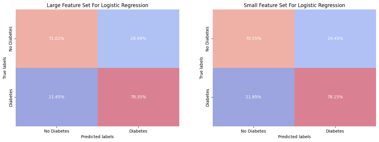
The models exhibit a demonstrates a reasonably ability in correctly identifying individuals with and without diabetes, with True Positive (sensitivity) rates of 78.35% for the larger feature set and 78.15% for the smaller feature set, and True Negative (specificity) rates of 71.01% and 70.55% respectively. However, in a potential clinical setting, the observed False Negative rates of 21.65% for the larger set and 21.85% for the smaller set could be of problematic, as they represent the proportion of actual diabetic patients who were not identified by the model. Same for the False Positive rates.

While the balance between precision and recall suggests that the models perform reasonably well for a general application, the consequences of false predictions in a medical context could be bad.

3.2 Decision Tree and Random Forest

df_train_trees = df_train.copy()
df_val_trees = df_val.copy()

dtype_dict_trees = {
    'int32': categorical_features + boolean_features
}

df_train_trees = convert_dtypes(df_train_trees, dtype_dict_trees)
df_val_trees = convert_dtypes(df_val_trees, dtype_dict_trees)


# For decision three is need only to select the feature matrix from dataframe
X_train_small, X_val_small =    df_train_trees[small_feature_list].values,\
                                df_val_trees[small_feature_list].values
                                
X_train_large, X_val_large =    df_train_trees[large_feature_list].values, \
                                df_val_trees[large_feature_list].values

3.2.1 Hyperparameter Tunning And Validate

Decision tree

# Decision Tree
param_grid = {
    'max_depth': [3 ,10, 15 ],
    'min_samples_split': [2, 5],
    'min_samples_leaf': [1, 8, 10],
    'criterion': ['gini']
}

dt = DecisionTreeClassifier(random_state = 42)
grid_search = GridSearchCV(dt, param_grid, cv=8, scoring='accuracy')
grid_search.fit(X_train_large, Y_train)

# Get best parameters and best score
best_params = grid_search.best_params_
best_score = grid_search.best_score_

print(f"Best Parameters: {best_params}")
print(f"Best Accuracy Score: {best_score}")

# Predict using best estimator
Y_pred_dt_large = grid_search.best_estimator_.predict(X_val_large)
print('\n Accuracy for Large Feature Set:', round(accuracy_score(Y_pred_dt_large, Y_val), 3))

# 'criterion': 'gini', 'max_depth': 10, 'min_samples_leaf': 10, 'min_samples_split': 2

Best Parameters: {'criterion': 'gini', 'max_depth': 10, 'min_samples_leaf': 10, 'min_samples_split': 2}

Best Accuracy Score: 0.7295637043271721

Accuracy for Large Feature Set: 0.732

dt_model_small = DecisionTreeClassifier(max_depth = 10, min_samples_leaf = 10,
                                        min_samples_split = 2,random_state = 42, criterion = 'gini')
dt_model_small.fit(X_train_small, Y_train)
Y_pred_dt_small = dt_model_small.predict(X_val_small)

print('Accuracy for Small Feature Set::',round(accuracy_score(Y_pred_dt_small, Y_val), 3))

Accuracy for Small Feature Set:: 0.735

Random Forest

# Define the hyperparameter grid
param_grid = {
    'max_depth': [10, 15, 20],
    'min_samples_split': [ 5, 10],
    'min_samples_leaf': [8, 10, 15, 20],
    'criterion': ['gini'],
    'n_estimators': [40, 50, 60],
    'n_jobs': [-1]  
}

# Instantiate the RandomForestClassifier
rf_model = RandomForestClassifier(random_state = 42)

# Perform GridSearch
grid_search = GridSearchCV(rf_model, param_grid, cv=10, scoring='accuracy')
grid_search.fit(X_train_large, Y_train)

# Retrieve best parameters and best score
best_params = grid_search.best_params_
best_score = grid_search.best_score_

print(f"Best Parameters: {best_params}")
print(f"Best Accuracy Score: {best_score:.3f}")

# Predict using the best estimator
Y_pred_rf_large = grid_search.best_estimator_.predict(X_val_large)
print('\n Large Model Accuracy:', round(accuracy_score(Y_pred, Y_val), 3))

# criterion': 'criterion': 'gini', 'max_depth': 20, 'min_samples_leaf': 15, 
# 'min_samples_split': 5, 'n_estimators': 60, 'n_jobs': -1

Best Parameters: {'criterion': 'gini', 'max_depth': 15, 'min_samples_leaf': 20, 
                    'min_samples_split': 5, 'n_estimators': 50, 'n_jobs': -1}

Best Accuracy Score: 0.745

Large Model Accuracy: 0.744

rf_model = RandomForestClassifier(max_depth=20, min_samples_leaf=15, min_samples_split=5, 
                                  n_estimators=60, random_state = 42, n_jobs=-1)
rf_model.fit(X_train_small, Y_train)
Y_pred_rf_small = rf_model.predict(X_val_small)

print('Small Model Accuracy:',round(accuracy_score(Y_pred_rf_small, Y_val), 3))

Small Model Accuracy: 0.747

3.2.2 Feature Importance

Feature importance in most tree-ensembles is calculated based an importance score. The importance score is a measure of how often the feature was selected for splitting and how much gain in purity was achieved as a result of the selection.

dt_model= DecisionTreeClassifier( max_depth = 10, min_samples_leaf = 10, min_samples_split = 2,
                                  random_state = 42, criterion = 'gini')

dt_model.fit(X_train_large, Y_train)

rf_model = RandomForestClassifier(max_depth=20, min_samples_leaf=15, min_samples_split=5, 
                                  n_estimators=60, random_state = 42, n_jobs=-1)

rf_model.fit(X_train_large, Y_train)

# Extract feature importance
importances_dt = pd.DataFrame( dt_model.feature_importances_ , 
                              index = pd.Index(large_feature_list, name='features'),
                              columns = ['feature_importance'])\
                              .sort_values(by='feature_importance', ascending=False)\
                              .reset_index()

importances_rf =  pd.DataFrame( rf_model.feature_importances_, 
                                index = pd.Index(large_feature_list, name='features'),
                                columns = ['feature_importance'])\
                                .sort_values(by='feature_importance', ascending=False)\
                                .reset_index()

fig, axes = plt.subplots(nrows=2, ncols=1, figsize=(10, 12))

# Plot Decision Tree Feature Importance
feature_threshold = 0.04
plot_feature_importance( df=importances_dt, x='features', y='feature_importance', ax=axes[0],
                         threshold=feature_threshold, title='Decision Tree', palette=[blue, red])

# Plot Random Forest Feature Importance
plot_feature_importance( df=importances_rf, x='features', y='feature_importance', ax=axes[1], 
                         threshold=feature_threshold, title='Random Forest', palette = [blue, red])

plt.tight_layout()
plt.show()

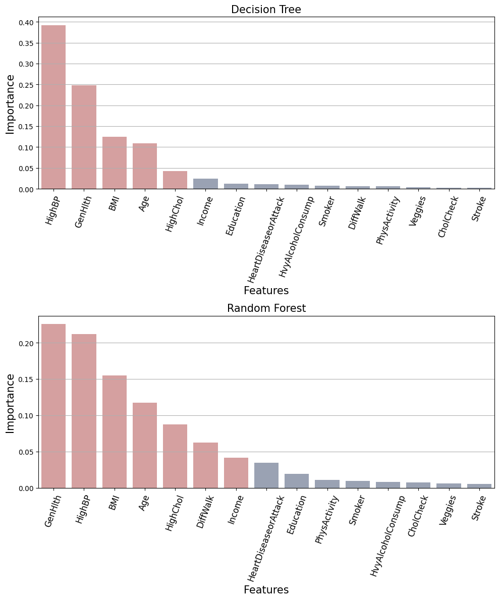
feature_importance_dt = set(
    importances_dt[importances_dt['feature_importance'] > feature_threshold]['features'])
feature_importance_rf = set(
    importances_rf[importances_rf['feature_importance'] > feature_threshold]['features'])

best_feature_set = feature_importance_dt.intersection(feature_importance_rf)\
                                        .intersection(feature_importance_lr)

print('Features importance Decision Tree:\n', feature_importance_dt)
print('\nFeatures importance Random Forest:\n', feature_importance_rf)
print('\nFeatures importance Logistic Regression:\n', feature_importance_lr)
print('\n Agreement between the three models:\n', best_feature_set)

Features importance Decision Tree:
 {'BMI', 'HighBP', 'HighChol', 'GenHlth', 'Age'}

Features importance Random Forest:
 {'BMI', 'HighBP', 'HighChol', 'Income', 'DiffWalk', 'GenHlth', 'Age'}

Features importance Logistic Regression:
 {'BMI', 'HighBP', 'HighChol', 'GenHlth', 'Age'}

 Agreement between the three models:
 {'BMI', 'HighBP', 'HighChol', 'GenHlth', 'Age'}

3.2.3 Metrics

dt_metrics_large = classification_metrics(Y_val, Y_pred_dt_large, 'dt_large_set')
dt_metrics_small = classification_metrics(Y_val, Y_pred_dt_small, 'dt_small_set')
dt_metrics = dt_metrics_large.merge(dt_metrics_small, on = 'metrics', how = 'outer')

rf_metrics_large = classification_metrics(Y_val, Y_pred_rf_large, 'rf_large_set')
rf_metrics_small = classification_metrics(Y_val, Y_pred_rf_small, 'rf_small_set')
rf_metrics = rf_metrics_large.merge(rf_metrics_small, on = 'metrics', how = 'outer')

trees_metrics = dt_metrics.merge(rf_metrics, on = 'metrics', how = 'outer')
display(trees_metrics)

	dt_large_set	dt_small_set	rf_large_set	rf_small_set
metrics
Precision	0.724642	0.728750	0.732304	0.731363
Recall	0.765897	0.768588	0.792664	0.798895
AUC	0.730749	0.734687	0.744799	0.745989
F1 Score	0.744698	0.748139	0.761289	0.763639

As we concluded for the logistic regression model, the smaller feature set provides almost equivalent performance to the larger set, specially for the F1 score and the recall metrics. which again suggests that the smaller feature set may contain the most relevant features.

predictions = {
    "Large Feature Set For Decision Tree ": Y_pred_dt_large, 
    "Small Feature Set For Decision Tree": Y_pred_dt_small,
    "Large Feature Set For Random Forest": Y_pred_rf_large,
    "Small Feature Set For Random Forest": Y_pred_rf_small  

}

# Create plots
fig, axes = plt.subplots(2, 2, figsize=((12, 8)))

for ax, (title, Y_pred) in zip(axes.ravel(), predictions.items()):
    plot_confusion_matrix(Y_val, Y_pred, title, ax, xy_legends=['No Diabetes', 'Diabetes'])

plt.tight_layout(pad=5.0)
plt.show()

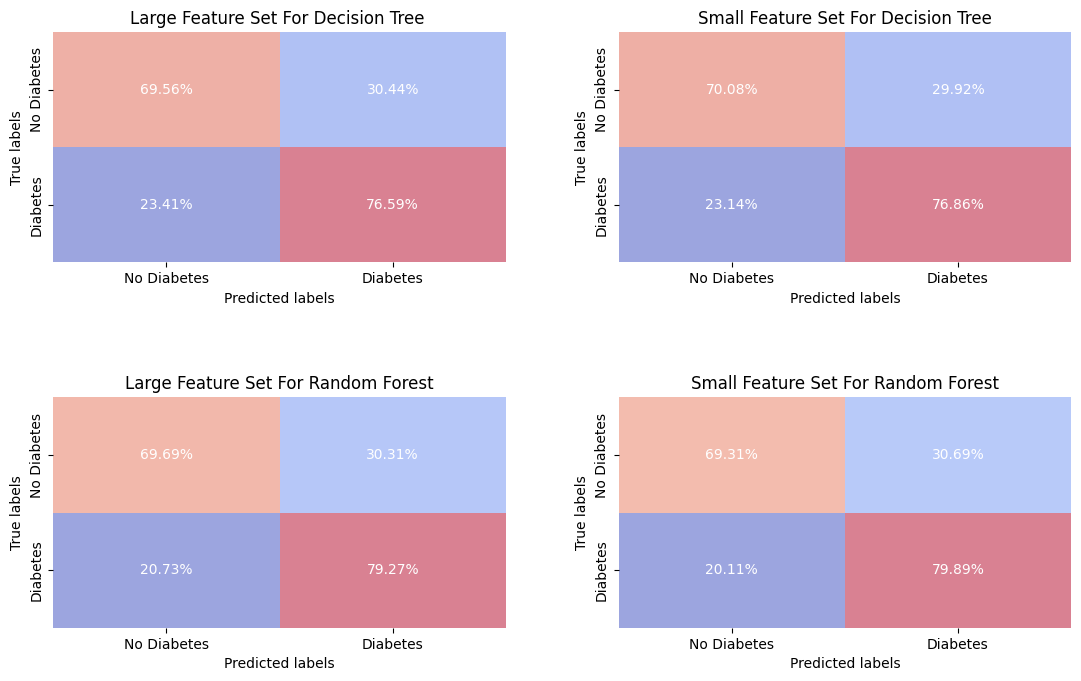
The Decision Tree and Random Forest models perform similarly for the different sets, with Random Forest showing a better predictive power in identifying true positives (correctly classify a diabetic individual) with 79.66%. The false negative rates are relatively low for all models, which is critical for a clinical test. This also confirm a suspected about redundancy in the larger feature set.

3.3 Selecting Model And Best Set Of Features

# Best set of features from the models
best_features_list = list(best_feature_set)

# Compare the difference between the sets of features
diff_feature_set = small_feature_set.difference(best_feature_set)

print('Features in small set but not in best set:\n', diff_feature_set)

Features in small set but not in best set:
 {'Income', 'DiffWalk', 'HeartDiseaseorAttack'}

 # Best set of features from the models
best_features_list = list(best_feature_set)

X_train_lr, X_val_lr, _, _ = model_train_preprocess(df_train_lr, df_val_lr, df_test_lr, best_features_list,
                                                                      dtype_dict_lr, features_to_scale=['BMI'])

X_train_trees, X_val_trees = df_train_trees[best_features_list].values, df_val_trees[best_features_list].values

# Logistic Regression
lr_model = LogisticRegression(solver = 'liblinear', penalty = 'l2', C = 1, random_state = 42)
lr_model.fit(X_train_lr, Y_train)
Y_pred_lr_best = lr_model.predict(X_val_lr)

#  Decision Tree
dt_model= DecisionTreeClassifier( max_depth = 10, min_samples_leaf = 10,
                                  min_samples_split = 2, criterion = 'gini',random_state = 42 )
dt_model.fit(X_train_trees, Y_train)
Y_pred_dt_best = dt_model.predict(X_val_trees)


# Random Forest
rf_model= RandomForestClassifier( max_depth=10, min_samples_leaf=10, min_samples_split=5, 
                                         n_estimators=60,criterion = 'gini', random_state = 42 ,n_jobs=-1)
rf_model.fit(X_train_trees, Y_train)
Y_pred_rf_best = rf_model.predict(X_val_trees)

predictions = {
    "Large Feature Set For Logistic Regression ": Y_pred_lr_large, 
    "Small Feature Set For Logistic Regression": Y_pred_lr_small,
    "Best Feature Set For Logistic Regression": Y_pred_lr_best,
    "Large Feature Set For Decision Tree ": Y_pred_dt_large, 
    "Small Feature Set For Decision Tree": Y_pred_dt_small,
    "Best Feature Set For Decision Tree": Y_pred_dt_best,
    "Large Feature Set For Random Forest": Y_pred_rf_large,
    "Small Feature Set For Random Forest": Y_pred_rf_small,
    "Best Feature Set For Random Forest": Y_pred_rf_best
}

# Create plots
fig, axes = plt.subplots(3, 3, figsize=(12, 12))

for ax, (title, Y_pred) in zip(axes.ravel(), predictions.items()):
    plot_confusion_matrix(Y_val, Y_pred, title, ax, xy_legends=['No Diabetes', 'Diabetes'])

plt.tight_layout(pad=5.0)
plt.show()

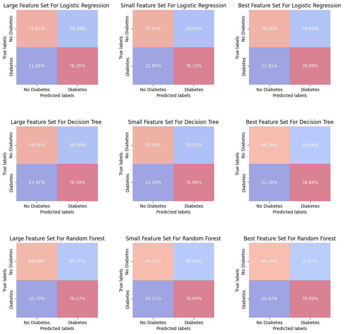
The best feature set consistently outperforms or matches the performance of the large and small feature sets in predicting both classes across all models! This is very good news, because implies that feature selection has been effective in improving model performance, reducing the complexity of the model.

One conclusion that we could drawn from this analyze is that the minor differences between the feature set performances may suggest that the models are somewhat robust to the features selected, or it may indicate that all sets contain the most critical features needed for making predictions.

lr_metrics_best = classification_metrics(Y_val, Y_pred_lr_best, 'lr_best_set')
dt_metrics_best = classification_metrics(Y_val, Y_pred_dt_best, 'dt_best_set')
rf_metrics_best = classification_metrics(Y_val, Y_pred_rf_best, 'rf_best_set')

metrics_best = lr_metrics_best.merge(dt_metrics_best, on = 'metrics', how = 'outer')\
                              .merge(rf_metrics_best, on = 'metrics', how = 'outer')

lr_metrics_large = classification_metrics(Y_val, Y_pred_lr_large, 'lr_large_set')
dt_metrics_large = classification_metrics(Y_val, Y_pred_dt_large, 'dt_large_set')
rf_metrics_large = classification_metrics(Y_val, Y_pred_rf_large, 'rf_large_set')

metrics_large = lr_metrics_large.merge(dt_metrics_large, on = 'metrics', how = 'outer')\
                                .merge(rf_metrics_large, on = 'metrics', how = 'outer')

metrics_small = lr_metrics_small.merge(dt_metrics_small, on = 'metrics', how = 'outer')\
                                .merge(rf_metrics_small, on = 'metrics', how = 'outer')

all_metrics = metrics_best.merge(metrics_large, on = 'metrics', how = 'outer')\
                          .merge(metrics_small, on = 'metrics', how = 'outer')
                           
display(all_metrics)

	lr_best_set	dt_best_set	rf_best_set	lr_large_set	dt_large_set	rf_large_set	lr_small_set	dt_small_set	rf_small_set
metrics
Precision	0.731688	0.722201	0.724752	0.738683	0.724642	0.732304	0.735145	0.728750	0.731363
Recall	0.780909	0.786433	0.795780	0.783458	0.765897	0.792664	0.781476	0.768588	0.798895
AUC	0.740699	0.735017	0.739839	0.746788	0.730749	0.744799	0.743500	0.734687	0.745989
F1 Score	0.755498	0.752949	0.758607	0.760412	0.744698	0.761289	0.757603	0.748139	0.763639

The minor differences between the metrics become clearer upon closer inspection. For example, the AUC values are quite close across all models, suggesting a consistent ability to distinguish between positive and negative classes. Furthermore, the F1 Score and Recall metrics indicate that the models excel at accurately identifying relevant cases with a low count of false negatives.

The most balanced model in terms of complexity and predictive power is the Random Forest with the best feature set, which contains only five features for this model.

4. Model Evaluation on Test Set

Next, we’ll evaluate the models on the test set. This step is important to confirm that the models’ performance is consistent with the validation results and to demonstrate their predictive stability on unseen data.

Logistic Regression

best_features_list = list(best_feature_set)

X_train_lr, _, X_test_lr, _ = model_train_preprocess(df_train_lr, df_val_lr, df_test_lr, best_features_list,
                                                    dtype_dict_lr, features_to_scale=['BMI'])


lr_model = LogisticRegression(solver = 'liblinear', penalty = 'l2', C = 1, random_state = 42)
lr_model.fit(X_train_lr, Y_train)
Y_pred_lr = lr_model.predict(X_test_lr)

accuracy_lr = accuracy_score(Y_test, Y_pred_lr)
print('Accuracy for Logistic Regression on test set:\n', round(accuracy_lr, 3))

Accuracy for Logistic Regression on test set:
 0.738

Decision Tree

# Best set of features selected from EDA
best_features_list = list(best_feature_set)

df_train_trees = df_train.copy()
df_test_trees = df_test.copy()

dtype_dict_trees = {
    'int32': categorical_features + boolean_features
}

df_train_trees = convert_dtypes(df_train_trees, dtype_dict_trees)
df_test_trees = convert_dtypes(df_test_trees, dtype_dict_trees)

# For decision three is need only to select the feature matrix from dataframe
X_train_best, X_test_best = df_train_trees[best_features_list].values,df_test_trees[best_features_list].values

dt_model = DecisionTreeClassifier(max_depth = 10, min_samples_leaf = 10,
                                        min_samples_split = 2,random_state = 42, criterion = 'gini')
dt_model.fit(X_train_trees, Y_train)
Y_pred_dt = dt_model.predict(X_test_best)

accuracy_dt = accuracy_score(Y_test, Y_pred_dt)
print('Accuracy for Decision Tree on test set:\n', round(accuracy_dt, 3))

Accuracy for Decision Tree on test set:
 0.731

Random Forest

rf_model = RandomForestClassifier(max_depth=20, min_samples_leaf=15, min_samples_split=5, 
                                  n_estimators=60, random_state = 42, n_jobs=-1)

rf_model.fit(X_train_trees, Y_train)
Y_pred_rf = rf_model.predict(X_test_best)

accuracy_rf = accuracy_score(Y_test, Y_pred_rf)
print('Accuracy for Random Forest on test set:\n', round(accuracy_rf, 3))

Accuracy for Random Forest on test set:
 0.734

 predictions = {
    "Logistic Regression On Validation Set": (Y_val, Y_pred_lr_best),
    "Logistic Regression On Test Set": (Y_test, Y_pred_lr),
    "Decision Tree On Validation Set": (Y_val, Y_pred_dt_best),
    "Decision Tree On Test Set": (Y_test, Y_pred_dt),
    "Random Forest On Validation Set": (Y_val, Y_pred_rf_best),
    "Random Forest On Test Set": (Y_test, Y_pred_rf)
}

fig, axes = plt.subplots(3, 2, figsize=(10, 10))

for ax, (title,  (Y_true, Y_pred)) in zip(axes.ravel(), predictions.items()):
        plot_confusion_matrix(Y_true, Y_pred, title, ax, xy_legends=['No Diabetes', 'Diabetes'])

plt.tight_layout(pad=5.0)
plt.show()

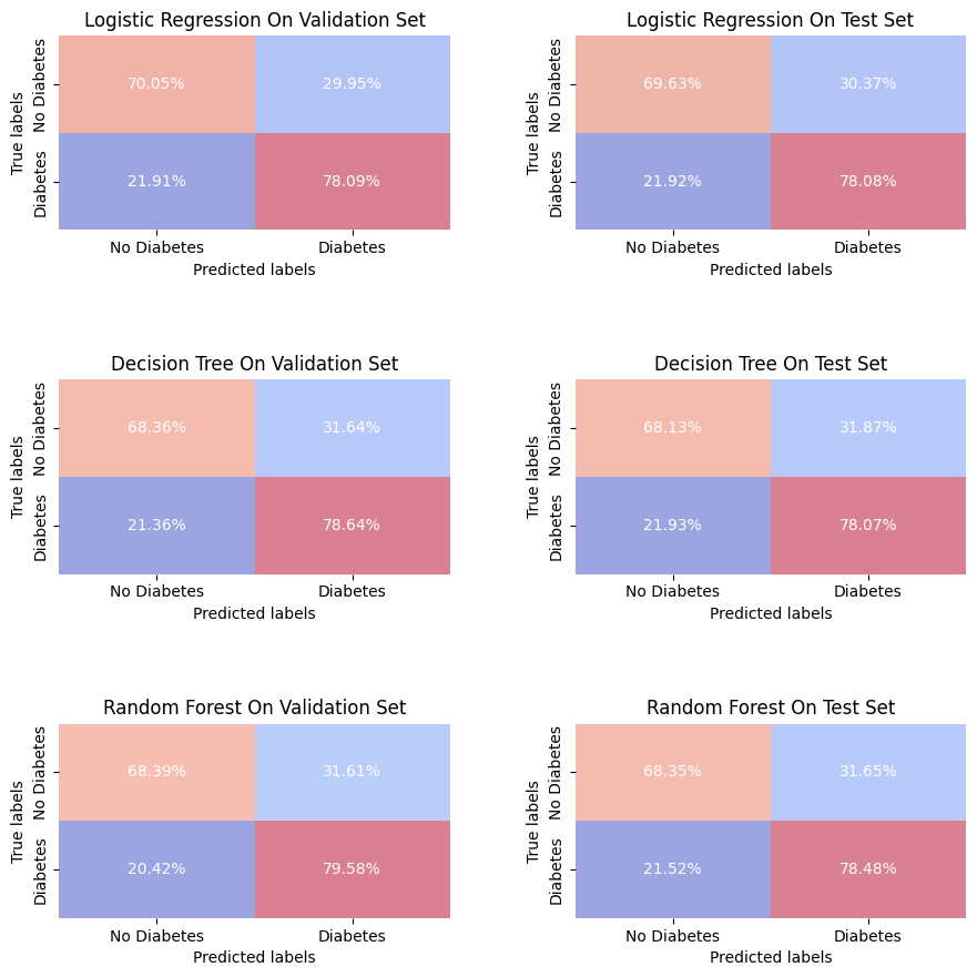
Each model shows a level of consistency between the validation set and test set, with only slight variations in the percentages of true positives (individuals correctly predicted with diabetes) and true negatives (individuals correctly predicted without diabetes), as well as false positives and false negatives. This suggests that the models are likely generalizing well and not overfitting to the validation data.

Also, we can note that the Random Forest model shows a high recall with a slight advantage in minimizing false positives (incorrectly predicts diabetes in an individual ), it could be considered the most stable model among the three, especially if the priority is to minimize false negatives.

5. Conclusions

From the exploratory data analysis (EDA), we identified the possibility of dropping some redundant features from the dataset out of the initial 22, leading to two subsets: the ‘small feature set’ (with features agreed upon by all correlation metrics) and the ‘large feature set’ (a union of features selected by both Mutual Information and Pearson Correlation).

In the Model Training and Validation section we showed that both feature sets produced similar outcomes across Logistic Regression, Decision Tree, and Random Forest models, with only slight variances in accuracy and other metrics such as F1 Score, Precision, Recall, and AUC. The Features selected by the models shows to be a even smaller set of feature, with only five features, that demonstrates also a high predictive power with only a marginal difference from the other features set.

The challenge in reducing the false negative rate (individuals wrongly classified with diabetes) from the different models may be due the possible skewed class distribution of the features CholCHeck, Stroke, HeartDiseaseorAttack, Vaggies, HvyAlcoholConsump, AnyHealthcare, NoDocbcCost, as noted previously in the EDA. One idea for improvement for the dataset in a future work may be focus on adding another tables from Kaggle that can be used complementary to the one used here.

A important information from our analysis is the indicative that the features BMI, GenHlth, Age, HighBP, and HighChol are the most predictive risk factors for diabetes, consistent with established clinical insights. Our project could reduce the feature space from 22 possible risk factors to just a subset of five, which simplified the predictive model without compromising accuracy.

The Random Forest model, using these five risk factors, proved to be the most balanced in terms of complexity and predictive capacity, and was selected for the final model deployment.

Marcos Benício

Marcos Benício

Analysis of Diabetes Indicators

Outline

1. Data Preprocessing

1.1. Split Dataset

2. Exploratory Data Analysis (EDA)

2.1 Feature Distribution

2.2 Feature Importance

2.3 Conclusion from EDA

3. Model Training and Validation

3.1 Logistic Regression

3.1.1 Hyperparameter tunning and validate

3.1.2 Feature importance

3.1.3 Metrics

3.2 Decision Tree and Random Forest

3.2.1 Hyperparameter Tunning And Validate

3.2.2 Feature Importance

3.2.3 Metrics

3.3 Selecting Model And Best Set Of Features

4. Model Evaluation on Test Set

5. Conclusions